Acoustic Modeling of Bangla Words using Deep Belief Network

Published Online September 2015 in MECS

Recently, speech recognition (SR) has drawn a great attraction to the research community due to its importance in human-computer interaction bearing scopes in many important tasks [1-2]. In general, SR is a system to transform naturally spoken words and phrases into machine-executable format. The basic units of a SR system are acoustic modelling (AM), language model and lexicon [3]. Among them, AM is crucial one which contains statistical representation of every distinct sound that makes up the word. Language model helps the SR system to figure out likelihood of word sequences independent of the acoustics; whereas, lexicon describes how words should be pronounced for SR.

A number of studies available from early 1990 to date for AM. Most of the SR systems use Hidden Markov Models (HMMs) [4-6] to deal with variability of the speech and Gaussian Mixture Model(GMM) [7-8] to determine how well the window of frames fit to each of the HMM state [9]. These methods are popular as they are easy to train theoretically, simpler and easy to decode. Later on Expectation Maximization (EM) algorithm [1011] introduced in SR systems for training HMMs. EM algorithm makes possible the SR process along with GMMs and also allows mapping acoustic input with the HMM state. But GMMs have several shortcomings. Firstly, GMM cannot model data that lie on the nonlinear state space, i.e., located close to the surface of a sphere. Secondly, they require a large number of diagonal Gaussians or full covariance Gaussians. With other shortcomings, GMMs are unable to acquire noticeable accuracy for complex structure of data due to their limited number of parameters and they model the state transition probability of HMMs quite roughly.

Artificial neural network (ANN) based methods are found as a good replacement of GMMs in SR system development [12]. H. Bourlard et al. [13] proposed a hybrid model, combination of HMMs and ANN for SR. In their model, they trained the ANN by back propagation algorithm to adjust the model parameters and model the data points that lie in the nonlinear space more accurately.

In recent years, a number of prominent SR methods have been developed using Deep Belief Network (DBN) [13-15]. DBN is a special type of ANN that contains many layers of non-linear hidden units (i.e., restricted Boltzmann machines) and a very large output layer. This large output layer is beneficial to accommodate large number of HMM states where each phone is modelled by different HMMs. A. R. Mohamed et al. [16] proposed an acoustic model using DBN for English SR on the Texas Instrumentsl Massachusetts Institute of Technology (TIMIT) database using monophone HMMs. The entire model has been learned with fixed or tied weights whereas each layer of RBMs has been learned by different weights. The authors show the effect of learning with different size of hidden layers and its subsequent contribution to the Phone Error Rate (PER). M. Zulkarneev et al. [17] proposed Russian SR using DBN in conjunction with HMM. Their recognition process consists of two stages. In the first stage DBN is used to calculate phoneme state probability and in the second stage Viterbi decoder is used to generate required sequence of words.

SR complexity varies among different languages due to different tones, accent and pronunciation. A number of prominent works, including the above discussed methods, are available for English and Russian with respect to other major languages such as Bangla. Bangla is one of the most largely spoken languages, ranked fifth in the world. It is the first language of Bangladesh and second most popular language in Indian subcontinent. However, the field of research in Bangla SR is at its early level. With almost 220 million Bangla speakers all over the world, there can be a lot of applications of SR.

A very few notable works are available for Bangla SR. M. A. Ali et al. [18] proposed four models for recognizing 100 Bangla words. They performed some pre-analysis on the speech signal such as applying high pass filter to discard the noise, Hamming window to integrate the closest frequency lines and FFT to decompress the signal into its constitute frequencies. G. Muhammad et al. [19] developed a SR system that recognizes Bangla digits using Mel Frequency Cepstral Coefficients (MFCC) and HMM based classifier. Their Bangla digit speech corpus comprises of native speakers but their system ends up in a confusion for few Bangla digits. M. A. Hossain et al. [20] presented Bangla SR system with ANN which is trained by back-propagation. In the system, extracted speech features using MFCC used to train ANN.

This paper proposes acoustic modeling of Bangla words using DBN combined with HMM for Bangla SR. MFCCs is used to accurately represent the shape of the vocal tract that manifests itself in the envelope of the short time power spectrum. Then DBN is trained with these feature vectors to calculate each of the phoneme states. After that Viterbi decoder is used to determine the resulting hidden state sequence that generates the word. The training of DBN is performed in two steps. In the first step, generative pre-training is used to train the network layer by layer with the output of one layer goes as the input of another layer. In the second step, enhanced gradient is used to slightly adjust the model parameters to make it more accurate. In addition, performance on training RBMs improved by adaptive learning, weight decay and momentum factor [21-22].

The rest of the paper is organized as follows. In Section II, we describe our proposed method to develop acoustic modeling for Bangla SR in detail. This section contains training the network and then fine tuning it to adjust the parameters. Section III is for experimental studies which contains simulation results of the proposed method and comparison with the existing related methods. In this section, we also presents how adaptive learning, weight decay and momentum factor improves the performance of the proposed model. Section IV presents some concluding remarks and future directions.

• II.    Acoustic Modeling of Bangla Words using Deep Belief Network (AMBW-DBN)

This section explains proposed AMBW-DBN in detail which has two major steps: speech data preparation and acoustic modeling using DBN. The DBN is first trained with real speech data and then fine-tuned with the training algorithms for multi-layered feed forward network. Finally, it is interfaced with HMM to predict the correct speech. The entire procedure is depicted below.

• A.    Speech Data Collection and Preprocessing

  The speech data have been collected from a relatively large number of native Bangla speakers. Speakers are asked to pronounce Bangla numerals “ ০ ( শূন )” to “ ৯ ( নয় )”. Such utterances have been used for fair comparison with the related works [20] although any Bangla utterances can be used to model the system. Forty-two speakers have been selected to cover the complete diversity i.e. age group, gender, literacy, area and language in which they generally speak. Each speaker has been asked to speak 10 words with 2 utterance of every word. Total 840 utterances (20 utterances for each speaker) of the words have been recorded. Speakers are asked to pronounce a word with about two seconds duration within a six seconds window period. Sampling frequency of 8192Hz has been used for this purpose. Table 1 shows the words with their Bengali and English pronunciation. The isolated words were recorded using two different microphones in front of computer.

Table 1. Bangla Numerals and Their Phonetic Pronunciation.

Bangla Numeral	Corresponding English Numeral	Bangla Utterance	English Phonetic
о	0	RR	Shunno
i	1		Ek
^	2		Dui
^	3	f^R	Tin
8	4	51^	Char
4	5	^tF	Pach
A	6	^5	Choy
Я	7	Rt»	Shat
t	8	^6 -	Aat
s	9	R5	Noy

Preprocessing eliminates the noise from the raw speech and converts the speech within actual boundary [23]. For the preprocessing purpose boundary detection algorithm [24] has been applied on the raw speech. The algorithm eliminated below 3db signal as considering noise. It also filtered raw speech into original spoken period within 2000ms. Fig. 1(a) shows the actual speech as it were recorded and Fig. 1(b) shows the processed speech by applying boundary detection algorithm on the recorded speech which is mainly used to model the system.

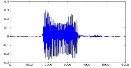
(a) Raw Speech

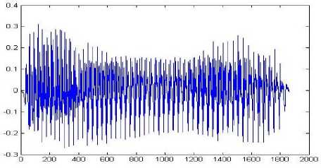
(b) Processed Speech

• B.    Acoustic Modeling (AM)

This section explains training of DBN with speech features which is collected from MFCC of the speech signal. After training, each of DBN’s RBM is fine-tuned to give better predictive performance. Finally, DBN has been interfaced with HMMs .

• B.1.    Training of Deep Belief Network (DBN)

DBN is a stack of restricted Boltzmann machines (RBMs) which is trained by layer-wise generative pretraining which is efficient as it allows discriminative fine tune to reduce over-fitting and to make rapid progress [25]. In generative pre-training, feature detectors of DBN are trained layer by layer and the output of one layer goes as the input of the next layer. Fig. 2 shows the example of training structure of DBN with three layers and an enlarged view of a RBM.

Fig.1. Sample Plot of Speech Signal.

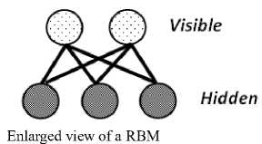
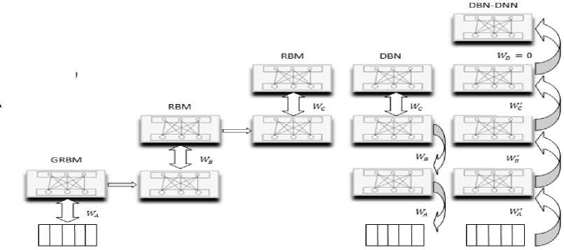
Fig.2. Training Structure of DBN with Three Layers of RBM with an Enlarged View of A RBM.

In this study, a seven layers of RBMs are considered for DBN and an efficient two stage training procedure is used. It starts by training RBMs containing stochastic binary visible units that represent the binary input data and connected to stochastic binary hidden units which represent the dependencies between the visible. Then the data inferred at the top RBM is goes as the input of the next RBM. This process is repeated until the seventh layer. Then the stack of RBMs is converted to a generative model where generated top-down directed connections are replaced by the lower level undirected connections.

RBM is an energy based model that has a structure similar to the bipartite graph, which means there is no direct connection between hidden-hidden and visible-visible units. It has visible units, which are represented by v and hidden units are represented by h , that can be inferred by the visible units and weight matrix W. The

smallest units of RBMs are stochastic binary units whose states are defined by Eq. (1).

p (v,h;W)=^e "E(y,h; ^),(1)

where Z is the partition function and works as a normalization factor. Z can be represented as

Z = E„Z he^E^\(2)

As RBM is an energy based model, the joint distribution of visible and hidden units has energy of the following form.

E(v, h) = -Et atvt - E bjhj - Eij vt hjWtj(3)

It is worth mentionable that negative energy is good. In the above i is the index of visible unit and j is the index of hidden unit. vi is the binary state of the visible unit and hjIs the binary state of the hidden units. Wy is weight connecting them. a is the visible unit bias and bj is the hidden unit bias.

The derivative of the log probability of a training set with respect to a weight is surprisingly simple.

^^ =< v_thj >_{d ata} -< v_thj > _moйе t     (4)

The derivation of the above equation gives a simple learning rule for the weight adjustments.

^AW ij = T ⁽ < Vh >< tata ^-< Vthj > mode i ),     ⁽⁵⁾

Where <  Vjbj > _data is Storage term in network and <  Vthj >_{m0d ei} is forget term to get rid of spurious minima and r) is the learning rate. The absence of any direct connections between visible and hidden units makes it useful to infer any unbiased sample < v_thj > _datn- The probability of binary state hj equal to 1 given any visible state is given by

p(hj = 1| v , W) = s igmoidbbj + E _i v _i W _i j )    (6)

Similarly the absence of direct connections also helps to infer the visible vector given the hidden one.

p(v = 1| h, W) = sigmoid(a _i + EthjW_t j )    (7)

However, getting the unbiased sample of <  v _i hj >_{mod e} i is very difficult. For this all the visible and hidden units have to be inferred at once that means above two equations must be evaluated for all the visible and hidden units in the network. This procedure is called Alternative Gibbs sampling.

Contrastive Divergence (CD) algorithm [26] gives a rough estimation of reconstructed binary units and offers an efficient training procedure implying increment of parameters. This starts by considering visible units as training vector. Then using Eq. (6) it computes hidden units which are in ON states given by the visible units. Then this hidden unit is used to calculate the visible units which are in ON states using Eq. (7). Thus the weight update rule is given by Eq. (8).

AW ij = (<< V_thj >_{d ata} -< vbj > reconstruction )  (8)

It’s essential that reconstruction should not depend on input vector , hence procedure of generating h and further reconstruction of is repeated several times.

In this study, an adaptive learning rate has been considered to improve the traditional DBN as suggested in [22]. Usually learning rate (p) of Eq. (8) is fixed. A set of learning rates are generated first and then the system is trained with one which gives minimum of energy and maximum likelihood. A batch wise operation was performed to select appropriate learning rate. Such batch- wise operation is important because it gives good indication about how well the data will fit on the next batch of training set or its performance on the current batch of data. At each step mini batch performs the computation of the gradient against more than one training examples [27]. This can perform significantly better than true stochastic gradient descent as it aggregates multiple examples at each iteration. It may also result in smoother convergence.

The weight update is further accompanied by concatenating a weight decay factor that reduces the chance of over-fitting. It involves adding a penalty term to the coefficient in order to discourage the coefficients from reaching large values. This yields the following update rule

A W ij =t [ < V i h >_data -< v_thj >_m o d e i- aWij ],    (9)

where is the weight decay factor.

The weight update is further influenced by “Momentum” which is useful as it smoothen the gradient. The idea consists of incorporating some influence of the past iterations in the present weight update.

AW ij = t [(1- P )V w _у,_t + VW_wu,t-1 ], 0 <  P < 1 (10)

where P is the momentum factor and V _wij>t, V _{Wlj> t}__T are the gradient calculated in current and previous iterations. The factor determines the amount of influence, previous iteration has on the current one.

As RBM is a binary stochastic unit and the feature vectors are in Gaussian form, we need a variant of RBM which can handle real valued data. GRBM is used to handle the real valued data by forming itself at the top layer of DBN [16]. RBM’s energy function can be modified to accommodate such variation, giving a Gaussian-Bernoulli RBM. Its energy function is of the following form.

E (V, h) = Ei (yp - Ej bbi - Ei, j ^ hj Wtj(11)

And the two conditional distributions required for CD algorithm are p (h7| v) = log isti c(_bj + E i” wi;-)(12)

p(Vi| h) = N (а + a^ihjWij ,Oi2)(13)

In the final stage, in order to calculate the posterior probability for interfacing with HMM, DBN is combined with DNN forming DBN-DNN [16]. DNN follows standard ANN architecture where the information in the layer ( ) below goes through the hidden units in the layer ( ) above.

Xj = ^bj+ ^E i yiWtj                ⁽¹⁴⁾

Vj = Sigmd id(x) =    ^_ _Xj          (15)

Apart from the elements with a Sigmoid function there is an output layer Softmax which operates as a transfer function, and produces probabilities that each of the HMM state should be in

(Zy ) Pi =∑к exp(Xk), where к is an index over all classes.

• B.2.    Fine Tuning of RBMs

After each of the RBM has been trained generatively, the next step is to adjust the model parameters slightly to achieve better predictive performance. An equivalent RBM can be obtained by flipping some bits and changing the weights and biases accordingly, but traditional learning rules are not invariant to such transformations. Without careful tuning of these training settings, traditional algorithms can easily get stuck or even diverge. In this letter, enhanced gradient is derived to be invariant to bit-flipping transformations. It yields more stable training of RBMs both when used with a fixed learning rate and an adaptive learning rate.

Normally the gradient can be calculated by the difference between the bias under model and bias under data. For example in case of visible bias visible_    _

=< visible _ bias >  data - <  visible _ bias > model (17)

The standard gradient has several potential problems. The gradients with respect to the weights contain the terms that point to the same direction as the gradient with respect to the bias terms and vice versa [11]. The standard gradient can be written as

∇ Wij = <  v_t >    ∇ Cj +<ℎ i >    ∇ b_t ,     (18)

where ∇Cj and ∇bt are hidden and visible bias gradients and <∙>  = <∙>d+ <∙> is the average activity of neuron under the data and model distributions.

• B.3.    Interfacing with HMM

Softmax layer is useful for providing the posterior probability, P ( state | Acousticinput ). In order to interface with HMM, it has to pass the likelihood, p ( Acousticinput | state ), as VD takes likelihood as its parameter. As it is known

Posterior ∝ Likeli ℎ ood ∗ Prior .       (19)

This prior probability can be roughly estimated as the probability that each of the state will be in. Generally this can be estimated as          for each of the state. As this

.of state term has no influence in the entire network it can be neglected and likelihood can be used as posterior. Finally, VD takes this probability and gives the most probable hidden state sequence that generates the observed output.

• C.    Significance of our proposed model

There are several significant differences among proposed AMBW-DBN and traditinal DBN based methods. A number of modification is introduced in RBM’s training. Firstly, the network is trained with adaptive learning rate, where the network automatically select a suitable learning rate among a set of generated learning rates and trained with it. Secondly, weight decay factor is used in order to avoid overfitting problem. Thirdly, a momentum factor is applied on the weight adjustment, which reduces reconstruction error. Finally, different parameters such as visible bias, hidden bias, weights etc. are adjusted using enhanced gradients.

• III.    Experimental Studies

This section first presents the experimental results with moderated analysis of the proposed AMBW-DBN and then outcome compares with the related exisiting methods. Performance is measured by varrying different parameters such as learning rate, no. of layers, no. of iterations, no. of speakers, momentum factor, gradients, and no.of HMM states. The accuracy is measured as the ratio of correct estimation to total estimation by VD.

• A.    Experimental Results and Analysis

  The AMBW-DBN system is implemented in Matlab2009a. The experiments has been conducted on Asus desktop machine (CPU: Intel Core i5 @ 3.20 GHz and RAM: 4.00GB) in windows 7 environment.

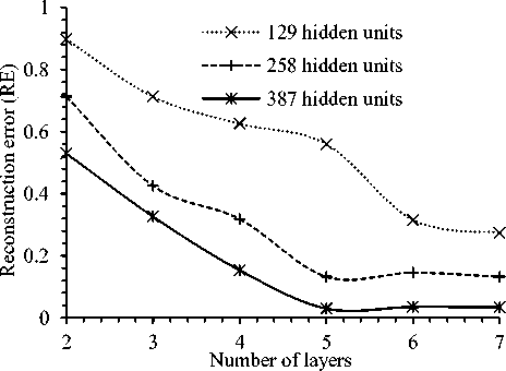
Fig.3. Reconstruction Error of Test Set Varying Number of Layers and Hidden Units per Layer.

At first, architecture of DBN is determined through experiments varying different number of layers and number of hidden units per layer. The number of layers varied from two to the maximum allowed number (i.e., seven). On the other hand, three different number of hidden units per layer which are 129, 258 and 387 are considered. The term reconstruction error (RE) influence performance of DBN and its minimum value indicates the appropriate architecture of a DBN. In general, RE is calculated by selecting the feature values through binomial distribution then sample the visible vector through sigmoid function. Later sum square error function is used to calculate the deviation of the reconstructed data from the model data. In the experiment, 560 samples of 28 speakers are used for training and rest 280 samples of other 14 speakers are used for testing purpose. Fig. 3 shows the RE on test set for varying different architectures. Form the figure it is observed that five layers with 387 hidden units in each layer gives minimum RE. This architecture are used for further experiments.

S3

BS= 100 (Test set)

BS = 100 (Training set)

BS = 200 (Test set)

BS = 200 (Training set)

Number of HMM states

Fig.4. Effect Of HMM States on Accuracy for Different Batch Size (BS).

Since number of HMM states is an element of accuracy, an experiment has been conducted to select appropriate number of the HMM states. Fig. 4 shows effect of HMM states on accuracy on both training and test sets for batch size (BS) 100 and 200. Samples in training and test sets were same as architecture determination experiment. According to the figure, accuracy on both training and test sets improved significantly up to five HMM sates for any batch size. Therefore, five HMMs states are considered for further experiments of AMBW-DBN. On the other hand, BS of 100 was considered like many existing studies.

л

Я g80

X--- AL = ON (Test set)

•X AL = ON (Training set)

'+--- AL = OFF (Test set)

......+..... AL = OFF (Training set)

50       70       90      110      130      150

Number of iteration

Fig.5. Effect of Training Iteration on Accuracy for With and Without Adaptive Learning (AL).

Number of iteration is an element for better learning and generalization in any learning system. Fig. 5 shows the effect of training iteration on accuracy for with and without Adaptive learning (AL). In case of without AL, the learning rate (LR) was fixed as of traditional methods and the value was fixed at 0.2. On the other hand, a set of LRs for each batch were generated based on the given fixed LR. For a particular batch, three LRs are generated from LR of the previous batch and training performed for this batch with the LR which gives minimum energy (Eq. (3)). For the first batch the three LRs are considered adding and subtracting 0.01 with given fixed LR value 0.2. According to the Fig. 5, AL always outperformed fixed LR for both learning (i.e., training set accuracy) and generalization (i.e., test set accuracy). From the Fig. 5 it is also observed that accuracy for all the cases improved significantly from 50 to 100 iterations and becomes fixed after that. Therefore, in further experiments number of iteration was considered as 100 with AL.

Finally, experiments conducted with AMBW-DBN considering five layers of RBMs, 387 units per layer and five HMM states trained for fixed 100 iteration with AL. The standard weight decay factor (i.e., the value of a in Eq. (9)) value 0.02 was considered in weight update. On the other hand, the momentum factor (i.e., the value of p in Eq. (10)) was considered as 0.9 on the basis of some trial runs. Table 2 shows the generalization ability (i.e., test set accuracy) of AMBW-DBN when tested in twofold and three-fold cross validation (CV) way for fair comparison with other works. In the two-fold CV 420 speech samples of 21 speakers (50% of the total samples) used for training and rest 420 samples of other speakers used for testing. The experiments were repeated two times interchanging training and test samples. On the other hand, in three-fold CV case the speech samples are divided into three parts and by turn one part, i.e., 280 samples of 14 speakers, is used as test set and rest 560 samples of 28 speakers was used as training set. According to the Table 2, the average accuracy for two-fold is 93.95% and best is 94.21% (test samples for Speaker 1 - 21). Accordingly, the average accuracy for three-fold is 92.42% and best is 93.23% (test samples for Speaker 29-42).

Table 2. Generalization Ability (I.E., Test Set Accuracy) of AMBW-DBN in Two and Three Folds Cross Validation Way.

Cross Validation (CV)	Train. Set: Fold wise Speaker	Test Set: Fold wise Speaker	Test set Accuracy
Two-fold : 420 samples for training and 420 samples for testing	Speaker 1–21	Speaker 22-42	93.69%
	Speaker 22-42	Speaker 1-21	94.21%
Two-fold average accuracy:			93.95%
Three-fold : 560 samples for training and 280 samples for testing	Speaker 1–28	Speaker 29-42	93.23%
	Speaker 1-14 and 29-42	Speaker 15-28	92.25%
	Speaker 29-42	Speaker 1-28	91.79%
Three-fold average accuracy:			92.42%

Table 3 shows the confusion matrix of test set having speech samples of speaker 29-42 in three-fold CV to understand which samples are misclassified as what. It is observed from the table that AMBW-DBN correctly identified all the test speech samples of S(Dui) and ^(Tin). On the other hand system performed badly for 6(Pach). Among 280 samples, 6(Pach) truly recognized in 276 cases and rest four cases it is recognized as R(Shat) and ^(Aat). The reason behind such misclassification is the variation of pronunciation of different speakers. To visualize the misclassification matter clearly, Table 4 presents frequency plot of few samples those are misclassified. Due to large variation in pronunciation among speakers such speech samples are difficult to correctly recognize even by human.

Table 3. Confusion Matrix of Test Set Having Speech Samples of Speaker 29-42 in Three-Fold Cross Validation.

	০ ( Shunno )	১ ( Ek )	২ ( Dui )	৩ ( Tin )	৪ ( Char )	৫ ( Pach )	৬ ( Choy )	৭ ( Shat )	৮ ( Aat )	৯ ( Noy )
০ ( Shunno )	279	0	0	1	0	0	0	0	0	0
১ ( Ek )	2	278	0	0	0	0	0	0	0	0
২ ( Dui )	0	0	280	0	0	0	0	0	0	0
৩ ( Tin )	0	0	0	280	0	0	0	0	0	0
৪ ( Char )	0	1	0	0	278	0	0	1	0	0
৫ ( Pach )	0	0	0	0	0	276	0	2	2	0
৬ ( Choy )	0	0	0	0	1	0	278	0	0	1
৭ ( Shat )	0	2	0	0	1	0	0	277	0	0
৮ ( Aat )	0	0	0	0	0	1	0	2	277	0
৯ ( Noy )	0	0	1	0	0	0	1	0	0	278

Table 4. Speech Samples that Are Misclassified by AMBW-DBN with Similar Speech Sample.

Misclassified speech sample	Almost similar speech sample for different numeral
*i*' 1 u зои ил ecu teu что паи i«xi ^t (Pach )	■: (^^ ^^ (Aat )
^ (Noy )	Hlfr1': С™П      IM     '№     ISM    ЗЯИ     MM ^(Choy )
■^ф||й ^t       2B0      -03      600       iBO      1033       ICO ^^ (Aat )	* *0 .ui шз er- ■ii чип ui» •■» Я|« (Shat)

• B.    Experimental Results Comparison

This section compares performance of the proposed AMBW-DBN with related methods. We have considered two recent studies of Bangla SR [18], [20] in performance comparison. Between the methods, Ref. [18] applied various signal processing techniques such as hamming window to integrate the closest frequency lines and FFT to decompress the signal into its constitute frequencies. On the other hand, Ref. [20] used MFCC to extract features and trained a NN with back propagation algorithm using these features. For better realization of the performance of the proposed method, we have implemented GMM-HMM [9], the widely used system for phoneme classification, and evaluated it with same speech samples of Bangla that we have collected.

Table 5. Comparison of Recognition Performance of Proposed AMBW-DBN with some Contemporary Methods of Bangla SR.

Methods	Data Set: Total Speaker/ Total Samples/ Test Samples	Test Set Recognition Accuracy	Remarks
M. A. Ali et al. [18]	- / 1000 / -	84.00%	Speech of 100 Bangla words
M. A. Hossain et al. [20]	10 / 300 / 150	92.00%	Speech of ten Bangla numerals ০ (Shunno) to ৯ (Noy)
GMM-HMM	42 / 840 / 420	87.75%
AMBW-DBN (Two-fold CV)	42 / 840 / 420	93.95%
AMBW-DBN (Three-fold CV)	42 / 840 / 280	92.42%

Table 5 compares the generalization ability (i.e., test set accuracy) among AMBW-DBN, GMM-HMM, and works of [18, 20]. The results of [18] and [20] are reported ones in the papers. Ref. [18] considered speech sample of 100 Bangla words but number of speakers and number of test samples used is not reported, therefore marked as “-” in data description column of comparison table. Ref. [20] considered total 300 speech samples of 10 Bangla numerals from ten speakers. Their result was followed as two-fold CV manner. The result of GMM-HMM also implemented in two-fold CV way with total 840 samples. On the other hand, the results of AMBW-DBN are collected from the Table 2. According to Table 5, our proposed AMBW-DBN outperformed other methods. GMM-HMM and [20] achieved 87.75% and 92.00%, respectively. Whereas, in two-fold case, the proposed method achieved recognition accuracy of 93.95%. Finally, the DBN based proposed AMBW-DBN revealed as an effective system for Bangla speech recognition.

• IV.    Conclusions

This paper proposes acoustic model for Bangla SR using DBN called AMBW-DBN which consists of multiple layers of feature detectors. Firstly, the system is trained by CD algorithm for multi-layered feed forward neural network. Then fine tuning fit the data to AMBW-DBN structure with some labelled information. In addition, accuracy is increased by applying adaptive learning rate, weight decay and momentum factor. Several experiments have been conducted with Bangla speech samples; and system’s performance are examined over various speaker subsets with different sex, age and dialect. Extensive analyses and results are presented to understand the effectiveness of the proposed method. The proposed AMBW-DBN outperformed other prominent methods when experimental results are compared with them.

A potential future direction is also opened from this study. The present study might be extended to develop acoustic model for continuous Bangla SR using recurrent NNs (i.e., Hopfield network). The Hopfield network greatly increases the amount of detailed information about the past that can be carried forward to help in the interpretation of the future [28].

Acknowledgment

The authors would like to show gratitude to Mikhail Zulkarneev (FSSI Research Institute Spezvuzautomatika, Rostov-on-Don, Russia) for his comments and sharing his pearls of wisdom during the course of this research.