Acoustic Signal Based Fault Detection in Motorcycles – A Comparative Study of Classifiers

Motorcycles are the obvious travel companions of middle-class Indians. The motorcycle sales dominate the Indian automobile market, accounting for nearly 77% of the vehicle sales [10]. Vehicle classification and fault diagnosis are the interesting applications of non-speech sound processing. The sound patterns produced by the vehicles indicate their working conditions and convey the information necessary for fault diagnosis. Different parts of the vehicles like rotating parts, crank, piston, timing chain, push rod and exhaust contribute to the generated sound. Expert mechanics assess the health condition of a vehicle based on the produced sound patterns. This trait of expert mechanics is the major motivation in developing automated fault diagnostic systems. However the research community has paid less attention for the fault diagnosis of motorcycles, despite the growth of motorcycle market in India and China. This current scenario made the authors to work on the fault diagnosis of motorcycles based on sound patterns.

The primary objective of this work is to detect the fault in motorcycles. A motorcycle detected as faulty gives a cue to the service mechanic to initiate suitable repair measures. The significant contribution made in this paper helps in automation of fault detection. Suitable repair in time avoids a major breakdown in the long run and aids for safety of the rider. The repair tips for the rider will help overcome the minor problems in remote places with rare expertise. The present work attempts to classify the motorcycles into healthy and faulty using temporal and spectral features. The extracted features are input to four different classifiers, namely DTW, ANN, k-NN and SVM independently. The study leaves scope for further investigation of faults in different subsystems and for hierarchical fault source localization. The literature on related works is reviewed to know the state-of-the-art and the survey is organized in three parts: non-speech sound recognition, vehicle classification and fault diagnosis.

Acoustic applications for musical instruments and heart sound analysis employ different feature sets and classifiers. Classification phase uses active learning probabilistic neural network (PNN). An extreme learning machine (ELM) is applied with an automatic segmentation algorithm for heart disorder classification [1]. A methodology is provided for automatic classification of bird species from the sounds produced by them using two-dimensional cepstral coefficients [2].

Some of the researchers employ different feature sets and variants of neural networks for vehicle classification. The conventional tools normally used for speaker recognition, namely, Mel-frequency cepstral coefficients (MFCC), Gaussian mixture models (GMM), hidden Markov models (HMM), are compared with the Bayesian subspace method based on the short term Fourier transform (STFT) for the acoustic signature analysis of the vehicles [3]. A backpropagation neural network for recognizing types of motorized two-wheelers is presented [4]. The time and frequency domain features are used as input for the neural network classifier.

Majority of the fault diagnosis applications employ time-frequency analysis of the signals. The 1D central contour moments and their invariants of wavelet coefficients are used as features [5]. Daubechie’s DB4 wavelet decomposition is carried out to extract the features. The extracted feature vectors are input for DTW classifier for fault detection of motorcycles. A fault diagnosis system is presented for a scooter engine by employing continuous wavelet transform (CWT) and artificial neural network [6]. The fault diagnosis of industrial robots dealt by [7] employs approximation and detailed coefficients of the wavelet for training a feedforward neural network. The fault recognition of gear vibration system based on intrinsic mode functions-autoregressive model (IMF-AR) and support vector machine (SVM) classifier [8]. A fuzzy reference model developed by [9] uses fuzzy self-organizing feature map to the data obtained from independent component analysis (ICA) for fault detection and diagnosis of industrial plant operation.

From the literature survey it is revealed that much of the research exists on broader level covering speech recognition, musical instrument recognition and medical diagnosis. The reported study for classification and fault detection of vehicles is almost negligible. Moreover the existing literature do not attempt for classification of motorcycle sounds in real-world environments. Use of simple features and classifiers in the present work make the approach suitable for real-time fault diagnosis. Ever increasing market for motorcycles in India and China and lack of on-board diagnostics for motorcycles motivated the study.

The remaining part of the paper is divided into four sections. The proposed methodology is discussed in Section II. The experimental results are presented in Section III. The Section IV presents a discussion on results with a comparative performance analysis of the classifiers. Finally Section V concludes the work.

• II.    Methodology

The problem in hand demands the processing of the samples recorded in real-world environment. Hence, the acquired sound samples are input for feature extraction without denoising. Figure 1 depicts the overview of the methodology. The proposed methodology comprises four stages namely, acquisition of sound samples, segmentation, feature extraction and classification. The sound samples of the motorcycles are acquired in authorized service stations under the supervision of expert mechanics. The acquired sound samples are segmented into segments of one-second duration for uniformity in processing. Temporal and spectral features are extracted over the segmented sound samples. The extracted features are input to the four different classifiers independently. The comparative performance analysis of the classifiers is presented.

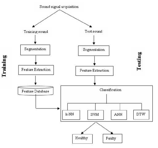
Figure 1. Block diagram of the proposed method

• A. Feature Extraction

The temporal and spectral behaviour of motorcycle sound patterns vary under different working conditions. Hence, the temporal features zero-crossing rate (ZCR), short-time energy (STE), root mean square (RMS) and spectral features mean and standard deviation of the spectral centroid (CMean and Csd) of the segmented sound samples are computed. These features are simple to use and compute. Following paragraphs explain the features in brief.

Time-Domain features: In speech recognition short time energy is used to discriminate between voiced and unvoiced speech signals. As signal energy values provide local information, they capture only short term characteristics. Short-time energy (STE) is a short-time speech measurement, which is defined as in (1).

m =w                   ²

E n = S t x ⁽ m ) w ⁽ n - ^{m ) ]}                         ( 1 )

m =—w

Zero-Crossing Rate (ZCR) is the rate of sign changes along a signal. It counts the number of zero crossings of a signal within the specified time interval. ZCR is a measure for the noisiness of a signal and is defined as given in (2).

m =w

Z„ = SI sign [ x ( m ) ] - sign [ x ( m — 1) ] w ( n - m )       ( 2 )

m =—w where w (n) =1N ,0 ^ n ^ N — 1.

Root mean square (RMS) is defined as the square root of the average of a squared signal in (3).

RMS

M

m = M — 1

E X 2 ( m )

where M is the total number of samples in processing window; x(m) is value of mth sample. It is used for endpoint detection of isolated utterances, voice activity detection and discrimination of speech and music. ZCR tends to be high in unvoiced sounds, whereas RMS is high in voiced sounds.

Frequency Domain Features: The ‘spectrum’ of frequency components is the frequency domain representation of the signal. The frequency domain provides an alternative description of sound in which the time axis is replaced by a frequency axis. Spectral centroid is based on the analysis of the frequency spectrum for the given signal. Generally spectral centroid is used to classify noise, speech and music. (4) defines the Discrete Fourier transform (DFT) to compute the spectrum.

lower end of the spectrum. Individually the features do not exhibit much separability for healthy and faulty samples, but in combinations, they do. Variations in the spectrum of the faulty samples may be attributed to the uneven operation of engine cycles in presence of faults, sound generated due to the damaged crank and leaky exhaust.

B. Classification

A ( n, k ) =

E x ( m ) w ( nL — M ) e

j ( 2 Г ^{) km}

where x(m) is the input signal, w(m) is a window function and L is the window length. The spectrum centroid is calculated as given in (5).

SC ( n ) =

z k =- 0 kA ( n , k ) 2i E K - o‘l ^{A (} n , ^{k ) 2}I

K is the order of DFT; k is the frequency for the nth frame, A (n, and k) is DFT of nth frame of a signal. The spectrum centroid indicates majority of high or low frequency content in the spectrum. The mean and the standard deviation of the spectral centroid are computed and used as features. The differences between the spectral features of healthy and faulty motorcycles lead to the classification of samples. The average power spectra of the sound signatures of healthy and faulty motorcycles are shown in Figure 2.

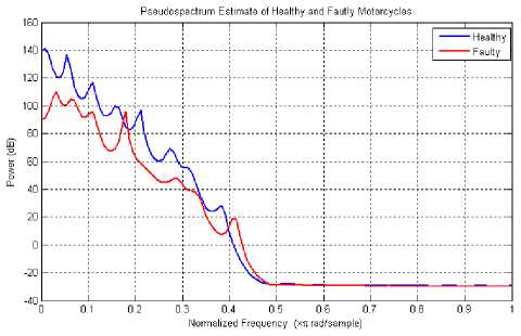
Figure 2. Average power spectra of sound signatures of healthy and faulty motorcycles

The classifiers classify the feature vectors derived from the sound samples into healthy and faulty. The chosen classifiers work on different principles. ANN-based classifier uses supervised learning. DTW computes the distance between the reference feature vectors and the test vectors. The smallest of the computed distances indicates the class. SVM classifier separates the test data into two groups, by trying to enlarge the gap between them. k-NN classifier computes the minimum of the distances between the current sample and the samples in the near vicinity. The features are combined by storing the individual feature values in an array of size five. The reference feature vectors of healthy samples are computed as the mean of the respective feature vectors of the healthy motorcycle samples. Similar procedure is followed to compute the reference feature vector for the faulty motorcycles.

ANN classifier [11]: An ANN is a mathematical model that tries to simulate the structure and functionalities of biological neural networks. Basic building block of every artificial neural network is artificial neuron, that is, a simple mathematical model (function). Such a model has three simple sets of rules: multiplication, summation and activation. At the entrance of artificial neuron the inputs are weighted i.e., every input value is multiplied with individual weight. In the middle section of artificial neuron is sum function that sums all weighted inputs and bias. At the exit of artificial neuron the sum of previously weighted inputs and bias is passing trough activation function. The error between the target and the obtained output is computed and is propagated back. The learning process adjusts the weights to minimize the error. Finally, the training ceases when the error is below the limits.

The validation process yielding the minimum mean squared error (MSE) is used to fix the number of nodes in the hidden layer. The neural network is trained using backpropagation-learning algorithm [13]. While testing, the stabilized weights are reloaded and the test vector is input. The optimal number of hidden layer neurons is chosen using the criterion [12] given in (6).

n = C

N d log N

The power spectrum of healthy motorcycles degrades uniformly and has no spurious spikes. But the variations in power spectrum of the faulty motorcycles are not uniform and some spurious spikes are observed in the

where, n=Number of hidden layer neurons, C=Constant to yield optimal performance, d=Number of features, and N=Number of rows in the training matrix.

MSE is computed for the sample sets with 70% of the samples used for training, 15% for validation and 15% for testing. The ANN is validated with number of

neurons varying from 3 to 15 in the hidden layer The minimum MSE is observed when 10 neurons are used in the hidden layer. Hence, the neural network is built to have 5 input nodes, 10 hidden layer nodes and 2 output nodes.

Dynamic Time Warping (DTW) [13]: The DTW measures the similarity of two sequences by warping them to find an optimal match. The algorithm matches the patterns independent of non-linear variations and sequences with unequal lengths. Suppose ms and mt are the reference and test feature vectors of lengths m and n respectively, the DTW algorithm finds an optimal distance.

The reference feature vector for healthy samples is computed as the mean of the respective healthy feature vectors. Similarly the reference feature vector for faulty samples is computed as the mean of the respective faulty feature vectors. DTW distances of the test feature vector with the healthy and faulty reference feature vectors are computed. If the DTW distance of the test feature vector to healthy reference feature vector is smaller than that of the faulty, the motorcycle is classified as healthy.

k-NN classifier: The k-NN classifier operates on the premises that classification of unknown instances can be done by relating the unknown to the known according to some distance function. An object is classified by a majority vote of its neighbors, with the object being assigned to the class most common amongst its k nearest neighbors, where k is a positive integer. If k = 1, then the object is simply assigned to the class of its nearest neighbor. The neighbors are taken from a set of objects for which the correct classification is known. The k-NN algorithm is sensitive to the local structure of the data.

SVM classifier: Given a set of training examples, each marked as belonging to one of two categories. The SVM takes a set of input data and predicts the possible class. An SVM model is a representation of the examples as points in space, mapped so that the examples of the separate categories are divided by a clear gap that is as wide as possible. New examples are then mapped into that same space and predicted as belonging to a category based on which side of the gap they fall on. It often happens that the sets are not linearly separable in the original finite-dimensional space. Hence such space will be mapped into a much higher-dimensional space, making the separation easier. The mappings used by SVM schemes are defined in terms of a kernel function K ( x , y ) selected to suit the problem. The training of SVM classifier involves the minimization of the error function given in (7):

N

_ wTw + C ^ _5i ( 7 ) ² i = 1

subject to the constraints: y (w^( x) + b )>1 - ^ and ^ > 0 , i = 1,2,„.,N where C is the capacity constant, w is the vector of coefficients, b a constant and ^ are parameters for handling nonseparable data. The index i labels the N training cases. Note that y e ±1 is the class label and x is the independent variable. The kernel ф is used to transform data from the input to the feature space. In our experiments, the performance of the classifier is tested with four kernel functions: linear, quadratic, polynomial and radial basis functions (RBFs).

• III.    Experimental results

  Sound samples of the motorcycles are recorded using Sony ICD-PX720 digital voice recorder under the supervision of expert mechanics. The sound sample database consists of recorded sound patterns of motorcycles of four major Indian motorcycle manufacturers. Motorcycles of different models from Hero Honda Motors Ltd., Honda Motorcycle and Scooter India Ltd., Bajaj Motors and T. V. Sundaram (TVS) Motor Co., are considered. Recorded sound samples are segmented into samples of one-second duration (with 44100 sample values). The sample set consists of 540 sound samples. It includes 270 samples of healthy motorcycles and 270 samples of faulty motorcycles.

• A.    Record ng env ronment and sound sample database

The recording is carried out in service stations, where external wind has least impact, but other disturbances from human speech, other motorcycles, air-compressor and auto-repair tools are common. Figure 3 depicts the recording environment. The recorder is held at 45o to the plane of the motorcycle at a distance of 500 mm. A circular area of 3 m radius around the motorcycle is left as an exclusion zone for all obstacles. Except the motorcycle under study, no other disturbances are allowed in this zone. In the outer circular zone of 5 m radius, the sound from other disturbances exists but does not exceed 80 dB (A).

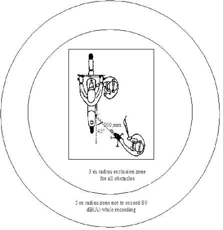
Figure 3. Recording environment

The engine runs in idling state while recording the sound patterns. The automotive standards suggest the use of sampling frequencies in the range of 9 kHz to 30 kHz, which is perfectly suitable for recording in an anechoic chamber with no surrounding noise. Since the real-world recording setup requires higher sampling frequencies, the sampling frequency of 44.1 kHz is used with 16-bit quantization. The acquired sound samples are segmented into samples of one second duration, for uniformity in processing. A segment begins at the local maxima in the first 50 ms duration of the time-domain signal. The features are extracted over the segmented samples without pre-processing.

MATLAB version 7.11.0.584 (R2010b) is used for effective implementation. Disjoint sets of samples are the 270 samples, n percentage ( n %) of the total samples is used for training, m percentage ( m %) for validation and the remaining samples are used for testing, where 30 ≤ n ≤ 50 and 20 ≤ m ≤ 35 , in steps of 5. The samples of the same motorcycle are not used for training as well as testing. The input feature values are divided into three subsets, based on the percentages chosen for training, validation and testing sets.

• B.    Performance of Dynamic time warping (DTW) classifier

The faults are detected based on the DTW distance of the test feature vectors with the reference feature vectors. DTW distances between test feature vector and the respective reference feature vectors of healthy and faulty samples are computed. The smallest of these distances indicates the condition of the motorcycle. If the DTW distance between a test vector and healthy reference vector is smaller than that between the faulty reference vector, then the test vector is classified as healthy. Figure 4 shows the DTW distances for healthy test feature vectors with the reference feature vectors of healthy and faulty samples. It can be observed that the DTW distances between healthy feature vectors with healthy reference vectors are smaller than those with the faulty reference vectors.

Comparison of healthy and faulty samples

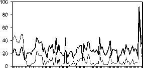
Healthy vs. Heatlhy

Healthy vs. Faulty

1  7 13 19 25 31 37 43 49 55 61 67 73 79 85 91 97

Samples

Figure 4. DTW distances for healthy and faulty motorcycles

The reference feature vectors are computed by averaging the training feature vectors column-wise. The classification performance is better in case of healthy motorcycles, which is evident from more True Positive (TP) cases than True Negative (TN) cases. This is mainly due to the uniformity of models chosen for healthy motorcycles. The faulty sample set has samples collected from different models of available motorcycles. Table 1 shows the classification performance by DTW classifier.

T able 1 C lassification performance of DTW classifier

% of Training samples	% of Validation samples	% of Test samples	Overall classification performance
			True Positive	True Negative	False Positive	False Negative	Accuracy
30	35	35	153	135	135	117	0.5333
35	35	30	197	151	119	73	0.6444
35	30	35	197	160	110	73	0.6611
40	35	25	215	167	103	55	0.7074
40	30	30	216	168	102	54	0.7111
40	25	35	216	180	90	54	0.7333
45	30	25	214	163	107	56	0.6981
45	25	30	214	162	108	56	0.6870
50	30	20	209	164	106	61	0.6907
50	20	30	209	158	111	62	0.6796
50	25	25	209	159	111	61	0.6815

DTW classifier yielded a maximum classification accuracy of 0.7333, which is not at appreciable for real-world situations. The computational cost of DTW algorithm is also discouraging. Further DTW is more suitable for applications where the recognition of speech in real-time or pass by vehicles, on-ride fault analysis, where the sequence changes with time. With increase in number of training samples, the performance does not increase consistently. Hence,

DTW is not a sensible classifier for this real-world problem.

• C.    Performance of ANN Classifier

  The simulation of the ANN is carried out in MATLAB version 7.11.0.584 (R2010b) for effective implementation. The classification performance of ANN depends on the learning rate, number of hidden layer neurons, extent of the training process and the number of epochs. The

performance of ANN classifier is tabulated in Table 2 for various combinations of training, validation and test sets. From Table 2 it can be observed that the best combination of training, validation and testing percentages is (40, 35, and 25) for better accuracy. The accuracies are appreciable. Since the dataset is roughly of size 500, and the features of the samples are extracted without denoising, the classifier has exhibited robust performance. The classification accuracy is observed to be more than 93% for this combination. Even for other combinations,

But the major problem with the ANN classifier is the time for training. Further, the time taken for training and the performance varies for every run, due to the random initialization of the weights. When the training halts, the error will be within the limits but by different extents. Hence the performance of the classifier is not uniform.

• D.    Performance of k-NN Classifier

k-NN classifier is tested with three values of neighborhood, k=1, k=2 and k=3 and for different distances. Figure 5 shows the classification accuracies for k-NN classifier with Euclidean distance, for k=1, k=2 and k-3.

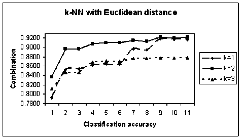
Figure 5. Classification performance of k-NN classifier for different values of k

It is clearly observed that the k-NN classifier yields better classification accuracy with k=2. Hence for this experiment, k=2 is chosen. Further it is necessary to analyze the performance of the classifier with different distance measures. Figure 6 shows the classification accuracies of k-NN classifier with k=2 and for different distance measures.

T able 2 C lassification accuracy with ANN classifier

% of Training samples	% of Validation samples	% of Test samples	Overall classification performance
			True Positive	True Negative	False Positive	False Negative	Accuracy
30	35	35	225	257	13	45	0.8926
35	35	30	215	262	8	55	0.8833
35	30	35	222	257	13	48	0.8870
40	35	25	244	261	9	26	0.9352
40	30	30	222	264	6	48	0.9000
40	25	35	221	263	7	49	0.8963
45	30	25	219	263	7	51	0.8926
45	25	30	221	259	11	49	0.8889
50	30	20	223	264	6	47	0.9019
50	20	30	222	266	4	48	0.9037
50	25	25	220	260	10	50	0.8889

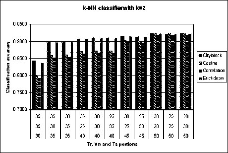
Figure 6. Performance for k-NN classifier with k=2 for different distances

From figure 6, the results are observed to be better with Cityblock distance compared to other distance measures. The results are consistently increasing with increasing number of training samples. This property is essential for the real-world situations. With increase in number of training samples, the classification performance increases. Cityblock distance and Euclidean distances have yielded consistent performance for almost all combinations of training, validation and test sets. The classification performance of k-NN classifier for different combinations of sample sets is shown in Table 3.

T able 3 C lassification performance of k -N earest N eighbour classifier

% of Training samples	% of Validation samples	% of Test samples	Overall classification performance k = 2 with Euclidean distance
			True Positive	True Negative	False Positive	False Negative	Accuracy
30	35	35	183	269	1	87	0.8370
35	30	35	215	269	1	55	0.8963
35	35	30	215	269	1	55	0.8963
40	25	35	220	269	1	50	0.9056
40	30	30	222	269	1	48	0.9093
40	35	25	221	269	1	49	0.9074
45	25	30	225	269	1	45	0.9148
45	30	25	224	269	1	46	0.9130
50	20	30	229	269	1	41	0.9222
50	25	25	229	269	1	41	0.9222
50	30	20	229	269	1	41	0.9222

• E.    Performance of SVM Classifier

SVM classifier is tested with different kernel functions. Figure 7 shows the performance of SVM classifier for different kernel functions.

parameters used with the classifiers. For e.g., the k-NN gives the best performance for k=2 with Cityblock distance. SVM has given the best performance with RBF kernel function. Hence the combined plot includes these results for the classifiers.

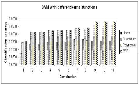
Figure 7. Performance for SVM classifier with different kernel functions

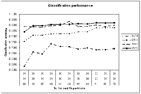
Figure 8. Overall performances of the classifiers

Among the kernel functions used (linear, quadratic, polynomial of degree three and RBF), the RBF has given the best performance compared to other kernel functions. It can be observed that quadrature kernel function yielded almost the same performance for all the combinations of inputs. But with increase in number of samples used for training, the performance suffers. For training sample sets of smaller sizes the performance is poor with the polynomial kernel function. Linear kernel function yielded poor classification accuracies for all the combinations. Hence the RBFs are inferred to be the suitable kernel functions with the SVM classifier for real-world noisy signal classification.

• IV.    Discussion

The performances of the classifiers differ for the larger training sample sets. The ANN classifier exhibits comparatively better performance for training sample sets of smaller sizes. Figure 8 shows the combined plot of classification performances of different classifiers. The results include the best accuracies that resulted for the

From figure 8, it can be clearly observed that k-NN classifier yields consistent performance. Major factors resulting in observable changes in sound are the deviation in engine operation cycles and exhaust noise due to improper combustion. DTW is practical for classifying samples with a limited database. Use of dynamic programming guarantees a polynomial complexity to the algorithm, O ( n ² v ) , where n is length of the sequence and v is the number of samples in the training set. The O ( n ² v ) complexity is not acceptable for a larger database. DTW is appropriate for applications with limited scope, for e.g., simple words recognition like reliability tests in manufacturing units, initial servicing activities in service stations, speech recognition in telephones, car computers, voice-based security systems and the like. Basic k-NN classifiers have a time complexity of о ( df |) where D is the size of the training set and F is the number of features, i.e., the distance metric is linear in the number of features and the comparison process increases linearly with the amount of data.

• V.    Conclusion

The presented work compares the performance of four classifiers for fault detection of motorcycles using acoustic signals. Simple temporal and spectral features are employed. From the empirical analysis, it is observed that the performances of k-NN, ANN, SVM and DTW are in the decreasing order, which means that the k-NN performed better than the other classifiers employed in this work. Computationally ANN is expensive than k-NN. Hence k-NN classifier is adjudged to be suitable in this work amongst the chosen classifiers. It is further observed that the performance varies based on the size of the sample sets chosen for training and larger training sets have given better accuracies. The work has scope for enhancement to fault source location in subsystems of vehicles. In addition it finds interesting acoustic-based fault diagnosis applications in industry, vehicles, civil constructions and the like.