Acoustic Signal based Traffic Density State Estimation using SVM

Density of traffic on roads and highways has been increasing constantly in recent years due to motorization, urbanization, and population growth. As the number of vehicle in urban areas is ever increasing, it has been a major concern of city authorities to facilitate effective control of traffic flows in urban areas [1]. Especially in rush hours, even a poor control at traffic signals may result in a long time traffic jam causing a chain of delays in traffic flows and also CO2 emission [2]. Intelligent traffic management systems are needed to avoid traffic congestions or accidents and to ensure safety of road users.

Traffic in developed countries is characterized by lane driven. Use of magnetic loop detectors, video cameras, and speed guns proved to be efficient approach for traffic monitoring and parameter extraction but the installation, operational and maintenance cost of these sensors significantly adds to the high operational expense of these devices during their life cycles. Therefore researchers have been developing several numbers of sensors, which have a number of significant advantages and disadvantages relative to each other. Nonintrusive traffic-monitoring technologies based on ultrasound, radar (Radio, Laser, and Photo), video and audio signals. All above present different characteristics in terms of robustness to changes in environmental conditions; manufacture, installation, and repair costs; safety regulation compliance, and so forth [3].

Traffic surveillance systems based on video cameras cover a broad range of different tasks, such as vehicle count, lane occupancy, speed measurements and classification, but they also detect critical events as fire and smoke, traffic jams or lost cargo. The problem of traffic monitoring and parameter estimation is most commonly solved by deploying inductive loops. These loops are very intrusive to the road pavement and, therefore cost associated with these is very high. Most video analytics systems on highways focus on counting and classification [4], [5], [6], [7], [8]. Using general purpose surveillance cameras for traffic analysis is demanding job. The quality of surveillance data is generally poor, and the range of operational conditions (e.g., night time, inclement, and changeable weather) requires robust techniques. The use of road side acoustic signal seems to be good approach for traffic monitoring and parameter estimation purpose having very low installation, operation and maintenance cost; low-power requirement; operate in day and night condition.

Support Vector Machine is most widely used neural network supervised learning model. SVM is used for the purpose of Classification and Regression. SVM does not have prior knowledge about problem but learns about it during training phase. Generalization capability is major advantage of SVM. This feature makes it better than most of the other models present in this field. To attain it right balance has to be maintained between the accuracy attained on the training data and the capacity of the machine [9]. SVM works equally for both linearly separable data as well as non-linearly separable data. The major advantage of SVM is its ability to classify unknown data set with high accuracy as it works on the concept of maximum margin hyperplane. Search of kernel function is not an easy task and it leads to major hurdle in the implementation of SVM. In order to get the best results, parameters of the kernel function have to be fine tuned. As different problems require different kernel functions, the choice of kernel function itself is a difficult task.

We start with a characterization of the road side cumulative acoustic signal which comprising several noise signals (tire noise, engine noise, air turbulence noise, and honks), the mixture weightings in the cumulative signal varies, depending on the traffic density conditions [10]. For low traffic conditions, vehicles tend to move with medium to high speeds, and hence, their cumulative acoustic signal is dominated by tire noise and air turbulence noise [10], [11]. On the other hand, for a heavily congested traffic, the acoustic signal is dominated by engine-idling noise and the honks. Therefore, in this work, we extract the spectral features of the roadside acoustic signal using Mel-Frequency Cepstral Coefficients (MFCC), and then SVM Classifier with various kernels are used to determine the traffic density state (low, Medium and Heavy).

We begin with description of the various noise signals in the cumulative acoustic signal in Section II. Overview of past work based on acoustic signal for traffic monitoring is provided in Section III, followed by feature extraction using Mel-Frequency Cepstral Coefficients in IV. Finally, the experimental setup and the classification results by SVM are provided in Section V, and the conclusion is summarized in Section VI.

• II.    V ehicular A coustic S ignal

A vehicular acoustic signal is mixture of various noise signals such as tyre noise, engine idling noise, noise due to exhaust, engine block noise, noise due to aerodynamic effects, noise due to mechanical effects (e.g., axle rotation, brake, and suspension), airturbulence noise and the honks. The mixture weighting of spectral components at any location is depends upon the traffic density condition and vehicle speed. In former case if we consider traffic density as freely flowing then acoustic signal is mainly due to tyre noise and air turbulence noise. For medium flow traffic acoustic signal is mainly due to wide band drive by noise, some honks. For heavy traffic condition the acoustic signal is mainly due to engine idling noise and several honks. Vehicular acoustic signals are summarized in TABLE. 1.

• III.    A coustic S ignals for traffic monitoring

Today’s urban environment is supported by applications of computer vision techniques and pattern recognition techniques including detection of traffic violation, vehicular density estimation, vehicular speed approximation, and the identification of road users. Currently magnetic loop detector is most widely used sensor for traffic monitoring in developing countries [21]. However traffic monitoring by using these sensors still have very high installation and maintenance cost. This not only includes the direct cost of labor intensive earth work but also, perhaps more importantly, the indirect cost associated with the disruption of traffic flow. Also these techniques require traffic to be orderly flow, traffic to be lane driven and in most cases it should be homogeneous.

Referring to the developing regions such India and Asia the traffic is non lane driven and highly chaotic. Highly heterogeneous traffic is present due to many two wheelers, three wheelers, four wheelers, auto-rickshaws, multi-wheeled buses and trucks, which does not follow lane. So it is the major concern of city authority to monitor such chaotic traffic. In such environment the loop detectors and computer-vision based tracking techniques are ineffective. The use of road side acoustic signal seems to be good alternative for traffic monitoring purpose having very low installation, operation and maintenance cost.

• A.    Vehicular Speed Estimation

Doppler frequency shift is used to provide a theoretical description of single vehicle speed. Assumption made that distance to the closest point of approach is known the solution can accommodate any line of arrival of the vehicle with respect to the microphone. [22], [23].

Sensing techniques based on passive sound detection are reported in [24], [25]. These techniques utilizes microphone array to detect the sound waves generated by road side vehicles and are capable of capable of monitoring traffic conditions on lane-by-lane and vehicle-by-vehicle basis in a multilane carriageway. S. Chen et Al develops multilane traffic sensing concept based passive sound which is digitized and processed by an on-site computer using a correlation based algorithm. The system having low cost, safe passive detection, immunity to adverse weather conditions, and competitive manufacturing cost. The system performs well for free flow traffic however for congested traffic performance is difficult to achieve [26].

Valcarce et al . exploit the differential time delays to estimate the speed. Pair of omnidirectional microphones was used and technique is based on maximum likelihood principle [3]. Lo and Ferguson develop a nonlinear least squares method for vehicle speed estimation using multiple microphones. Quasi-Newton method for computational efficiency was used. The estimated speed is obtained using generalized cross correlation method based on time-delay-of-arrival estimates [27].

Cevher et al. uses single acoustic sensor to estimate vehicle’s speed, width and length by jointly estimating acoustic wave patterns. Wave patterns are approximated using three envelop shape components. Results obtained from experimental setup shows the vehicle speeds are estimated as (18.68, 4.14) m/s by the video camera and (18.60, 4.49) m/s by the acoustic method [28].

• B.    Traffic Density Estimation

Time estimation for reaching from source to destination using real time traffic density information is major concern of city authorities. J. Kato proposed method for traffic density estimation based on recognition of temporal variations that appear on the power signals in accordance with vehicle passes through reference point [29]. HMM is used for observation of local temporal variations over small periods of time, extracted by wavelet transformation. Experimental results show good accuracy for detection of passage of vehicles

• IV.    FEATURE EXTRACTION USING MFCC

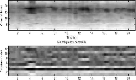
  An omnidirectional microphone was placed on the pedestrian sidewalk at about 1 to 1.5 m height, and it recorded the cumulative signal at 16000 Hz sampling frequency. Samples were collected for time durations of around 30s for different traffic density state conditions (low, medium and heavy). The various traffic density states induce different cumulative acoustic signals. To prove the above statement, we have examined the spectrogram of the different traffic state’s cumulative acoustic signals.

• •    For the low density traffic condition in Fig. 1, we only see the wideband drive-by noise and the air turbulence noise of the vehicles. No honks or very few honks are observed for low density traffic condition.

• •    For the medium density traffic condition in Fig. 2, we can see some wideband drive-by noise, some honk signals, and some concentration of the spectral energy in the low-frequency ranges (0, 0.1) of the normalized frequency or equivalently (0, 800) Hz.

• •    For the heavy density traffic condition in Fig. 3, we notice almost no wideband drive-by engine noise or air turbulence noise and are dominated by several honk signals. We note the several harmonics of the honk signals, and they are ranging from (2, 6) kHz.

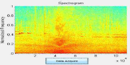
Figure. 1 Spectrogram of the low density traffic (above 40 km/h).

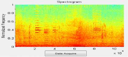
Figure. 2 Spectrogram of the Medium density traffic (20 to 40 km/h).

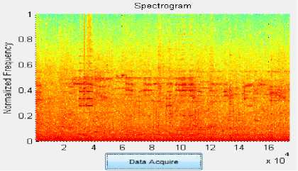
Figure. 3 Spectrogram of the Heavy density traffic (0 to 20 km/h).

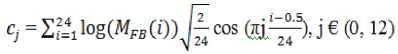
The goal of feature extraction is to give a good representation of the audio tract from its response characteristics at any particular time. Mel-Frequency cepstral coefficients (MFCC), which are the Discrete Cosine Transform (DCT) coefficients of a Mel-filter smoothed logarithmic power spectrum. First 13–20 cepstral coefficients of a signal’s short time spectrum succinctly capture the smooth spectral envelope information. We have decided to use first all the cepstral coefficients to represent acoustic signal for corresponding traffic density state. These coefficients have been very successfully applied as the acoustic features in speech recognition, speaker recognition, and music recognition and to vast variety of problem domains. Features extraction using MFCC is as follows,

• A.    Pre-emphasis

Pre-emphasis phase emphasizes higher frequencies. The pre-emphasis is a process of passing the signal through a filter. It is designed to increase, within a band of frequencies, the magnitude of some frequencies (higher) with respect to the magnitude of the others frequencies (lower) in order to improve the overall SNR.

y[n]= x[n]-αx[n-1], α € (0.9, 1) (1)

Where x[n] denotes input signal, y[n] denotes output signal and the coefficient α is in between 0.9 to 1.0, α= 0.97 usually. The goal of pre-emphasis phase is to compensate high-frequency part that was suppressed during the sound collection.

• B.    Framing and Windowing

Typically, speech is a non-stationary signal; therefore its statistical properties are not constant across time. The acquired signal is assumed to be stationary within a short time interval. The input acoustic signal is segmented in frames of 20~40 ms with overlap (optional) of 1/3~1/2 of the frame size. In order to keep the continuity of the first and the last points in the frame, typically each frame has to be multiplied with a hamming window. Its equation is as follows,

F (Mel) = 2595 * log 10 [1+f/700]

The i th Mel-filter bank energy (M FB (i)) is obtained as

W[n]= J 0.54 - 0.46cos — ,0 <  n <  N     (2)

I 0, otherwise N

Where N is frame size

Y[n]= X[n] * W[n]                              (3)

Where Y[n] = Output signal

X[n] = Input signal

W[n] = Hamming Window

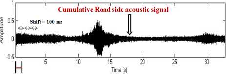
Due to the physical constraints, the traffic density state could change from one to another (low to medium flow to heavy) over at least 5–30 min duration. Therefore, we decided to use relatively longer primary analysis windows of the typical size 500 ms and shift size of 100 ms to obtain the spectral envelope.

Speech waveform

Primary Window

= 500 ms

Figure. 4 Primary windows of size=500 ms and shifted by 100 ms to obtain a sequence of MFCC feature vectors.

• C.    DFT

Commonly, Fast Fourier Transform (FFT) is used to compute the DFT. It converts each frame of N samples from time domain into frequency domain. The computation of the FFT-based spectrum as follow,

-jinnk

X[k] =                                        (4)

Where N is the frame size in samples, x[n] is the input acoustic signal, and. X[k] is the corresponding FFT-based spectrum.

• D.    Triangular bandpass filtering

The frequencies range in FFT spectrum is wide and acoustic signal does not follow the linear scale. Each filter’s magnitude frequency response is triangular in shape and is equal to unity at the Centre frequency and decrease linearly to zero. We then multiply the absolute magnitude of the DFT samples by the triangular frequency responses of the 24 Mel-filters that have logarithmically increasing bandwidth and cover a frequency range of 0–8 kHz in our experiments. Each filter output is sum of its filtered spectral components. To compute the Mel for given frequency f in HZ, equation is as follows:

№b (0) = (Meli №)) *№)|², к € (0, №)

Where (Mel i (k)) is the triangular frequency response of the i th Mel-filter. These 24 Mel-filter bank energies are then transformed into 13 MFCC using DCT.

• E.    DCT

This is the process to convert the log Mel spectrum into time domain using DCT. The result of the conversion is called Mel Frequency Cepstral Coefficient. The set of coefficient is called acoustic vectors.

• F.    Data energy and Spectrum

The acoustic signal and the frames changes, such as the slope of a formant at its transitions. Therefore, there is need to add features related to the change in cepstral features over time. Ex. 13 feature (12 cepstral features plus energy).

Energy=∑ X ² [t]

Where X[t] = signal

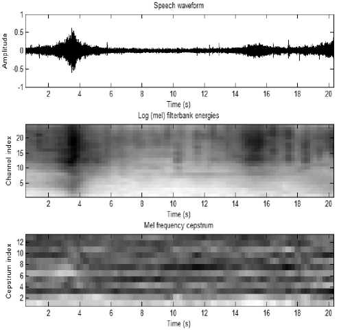
Figure. 5 Input Acoustic signal, corresponding log filterbank energies and Mel frequency cepstrum for low traffic density state

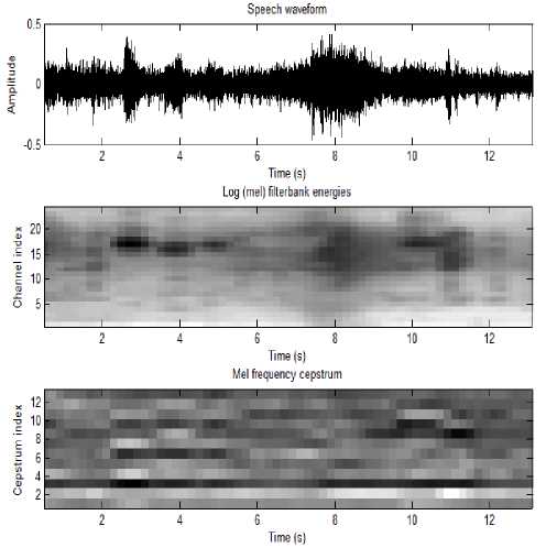
Figure. 6 Input Acoustic signal, corresponding log filterbank energies and Mel frequency cepstrum for Medium traffic density state

separate the various classes with a high margin [30]. Therefore SVM is proved to be excellent classifiers for diverse pattern recognition applications such as handwritten digit recognition [31], object detection [32], speaker recognition [33], etc. In general, a non-linear SVM projects the d-dimensional input features to some high-dimensional space H through a non-linear transform Φ.

Φ：Rd

-

→H

Time (s)

Log (mel) filterbank energies

The SVM composes the transformation Φ and the dot product in the higher dimensional space into a single kernel function k, which computes the dot product of two vectors when they are transformed into the higher space. Note that the kernel need not actually do any transformation to provide this dot product! This is called the kernel trick.

A. Building the Hyperplane

Consider the input data in the form (x i _,y i ), where vectors x i are in real-valued multi-dimensional space H and y i are the class labels. So any hyperplane is defined as

{ % E /Y|  + b=0} W € /V^ b E R (10)

Time (s)

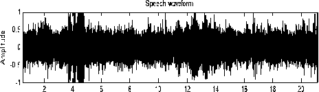
Figure. 7 Input Acoustic signal, corresponding log filterbank energies and Mel frequency cepstrum for Heavy traffic density state

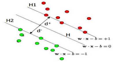
Figure. 8 Hyperplane through two linearly separable classes

Hyperplane is defined such that xi . w + b ≥ +1 when = +1

x _i . w + b ≤ -1 when = -1

And minimize ||w|| ²

H1 and H2 are the planes:

H1:   x i . w + b = +1

H2:   x i . w + b = -1

• V.    SVM CLASSIFIER

A Linear Support Vector Machine (SVM) uses linear decision boundary. But in case of non-separable data set, linear SVM is not very effective in classification. SVMs build a hyperplane which divides samples such that samples of one class are all on one side of the hyperplane, and samples of the other class are all on the other side. However, data is rarely linearly separable. Thus, SVM project the data in a high-dimensional space, where the classification problem may be linearly separable, and then find the linear hyperplanes that

The points on the planes H1 and H2 are the support vectors.

d+ = the shortest distance to the closest positive point d- = the shortest distance to the closest negative point

The margin of a separating hyperplane is d+ + d-.

Non Linear SVM: In the Linear SVM, to classify the training set a linear decision boundary is used. In case of non-separable data, the data set is not completely classified by linear decision boundary. Non-separable points can be classified correctly by using non-linear decision boundary. In general, models are not scalable from linear region to non-linear region but SVM can be converted from linear to non-linear mode with few changes. Non-linear SVM employs a non-linear decision function to classify the training data set by mapping the non-separable data points to higher dimension space where these data points become separable. In non-linear SVM, decision function will depend on Φ (xi) ∙ Φ (xj) instead of xi . xj So, the

• B.    Decision function

f ⁽ x ) = Ti ^ ^{1 (} x i ) ®⁽ x ) + ^Ь

= Т « i k ( X i , x ) + b                   (11)

• C.    Dual Formulation

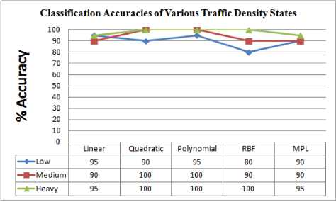
  TABLE. 3 Classification Accuracies of Various Traffic Density States

  
  
  
  
  
  
  
  

Where                maximize the margin and minimize the training error.

Can also be written as mi^D (K) = " Sy oc^. ФО-Ф (Xj) - ^у, «г such that Si ai =0 and 0 ^ 7i “t^ C

Kernel function K( , ) is used to make non linear feature map.

TABLE. 2 SVM kernels and kernel functions

Kernel	Kernel functions
Linear	К (x,xj) = xtTx
Quadratic	K(x,Xt) = (xXrT + I)2
Polynomial	К (xfXi) = (x xtT + 1/
REF	К (х,х,)= exp (-y|| x — x, |p)
MLP	K(x,Xj^tanh (кхх^хх^ + б)

• D.    Experimental Results

We have collected the road side cumulative acoustic signal samples from chhatrapati square to T-point of Nagpur city. Data were collected with 16 KHz sampling frequency. These data covered three broad traffic density classes (low, medium and heavy). Feature extraction is done using MFCC where primary window size is 500 ms and shift size is of 100 ms. Based on extracted features different kernel functions of SVM were used for the classification which results in classification accuracy as follows,

• VI.    C onclusion

This paper describes a simple technique which uses MFCC features of road side cumulative acoustic signal to classify traffic density state as Low, Medium and Heavy using different kernel functions of SVM. As this technique uses simple microphone (cost: 500 Rs) so its installation, operational and maintenance cost is very low. Technique works well under non lane driven and chaotic traffic condition, and is independent of lighting condition. Acceptable Classification accuracy is achieved using SVM classifier. Experimental results show that 96.67% and 98.33% classification accuracy obtained using quadratic and polynomial kernel functions respectively when entire cepstral coefficients were considered.

The research on vehicular acoustic signal which is mixture of engine noise, tyre noise, noise due to mechanical effects etc. expands from vehicular speed estimation to density estimation. The use of road side acoustic signal seems to be an alternative, research shows acceptable accuracy for acoustic signal. Vehicular classification with Acoustic signals proved to be excellent approach particularly for battlefield vehicles, and also for city vehicles.

Acknowledgment