Action-Dependent Adaptive Critic Design Based Neurocontroller for Cement Precalciner Kiln

Published Online October 2009 in MECS

As the world's largest cement production nation, cement production in China is still in an important phase of industrial restructuring. At present about half of the cement on the market is produced using the traditional methods (shaft, wet rotary kiln) and the other half using the newer precalciner kiln (PCK) system. To promote the new dry kiln technology, and eliminate the large energy consumption of shaft kiln and wet rotary kiln at the same time, we should further explore optimization methods for the new dry kiln technology to lower energy consumption and guarantee the safe and orderly production of cement.

In this paper, a new type of optimization technology -Adaptive Critic Design is used in the PCK system production control. From the perspective of a number of

Manuscript received January 12, 2009; revised July 21, 2009; accepted July 17, 2009.

balances about cement production, that is, the material balance, gas balance and heat balance, this paper wants to optimize the production of cement, and to further improve the efficiency and stability.

• II.    Framework of the ACD Method

Cassical dynamic programming is the only exact and efficient method to compute the optimal control policy over time, in a general nonlinear stochastic environment. From the versions developed by Howard [1] and Bertsekas [2] , dynamic programming can find optimal solution of general MIMO nonlinear system in theory, it can conquer the feedback caused by undermined factors. However, Dynamic programming may cause difficulties when it computes and save in memory, especially for high dimension system which may case curse of dimension. In fact, the real application of Dynamic programming need to be Approximate, e.g. the Adaptive Critic Design mentioned in this paper. ACD use approach function to express cost-to-go function, which avoid curse of dimension [3]. The only reason to approximate it is to reduce computational cost, so as to make the method affordable (feasible) across a wide range of applications.

• A.    Dynamic Programming of discrete-time nonlinear (time-varying) system

Suppose that one is given a discrete-time nonlinear (time-varying) dynamical system x (t +1) = F [ x (t), u (t), t ], t = 0,1,2, K l    (1)

where x G R n represents the state vector of the system and u G R^m denotes the control action. Suppose that one associates with this system the performance index (or cost)

«

J [ x ( i ), i ] = E Y - i U [ x ( k ), u ( k ), k ]      (2)

k = i where U is called the utility function and у is the discount factor with 0 < у < 1 . Note that the function J is dependent on the initial time i and the initial state

x ( i ) , and it is referred to as the cost-to-go of state x ( i ) . The objective of the dynamic programming problem is to choose a control sequence u ( k ), k = i , i + 1, к , l so that the function J (i.e., the cost) in (2) is minimized. Dynamic programming is based on Bellman’s principle of optimality: An optimal (control) policy has the property that no matter what previous decisions have been, the remaining decisions must constitute an optimal policy with regard to the state resulting from those previous decisions.

Suppose that one has computed the optimal cost J [ X ( t + 1), t + 1] from time t + 1 to the terminal time, for all possible states X ( t + 1) , and that one has also found the optimal control sequences from time t + 1 to the terminal time. The optimal cost results when the optimal control sequence u ( t + 1), u ( t + 2), к , is applied to the system with initial state X ( t + 1) . Note that the optimal control sequence depends on X ( t + 1) . If one applies an arbitrary control u ( t ) at time t and then uses the known optimal control sequence from t + 1 on, the resulting cost will be

J [ X ( t ), t ] = U [ X ( t ), u ( t ), t ] + y J * [ x ( t + 1), t + 1] (3)

where X ( t ) is the state at time t , and X ( t + 1) is determined by (1). According to Bellman, the optimal cost from time t on is equal to

J * [ X ( t ), t ] = min{ U [ x ( t ), u ( t ), t ] u ( t )

+ y J * [ x ( t + 1), t + 1]}

The optimal control u * (t) at time t is the u(t) that achieves this minimum, i.e., u *( t) = argmin{U [ x (t), u (t), t ] u(t)

+ y J [ x ( t + 1), t + 1]}

So the solution for u ^* ( t ) becomes a simple optimization problem.

• B.    The basic structure and principle of Adaptive Critic Design

The ACD technique, which was proposed by Werbos [4], is a novel optimization and control algorithm based on the mathematical analysis to handle the classical optimal control problem by combining concepts of reinforcement learning and dynamic programming. Use of the ACD technique allows the design of an optimal adaptive nonlinear controller [5].

In the development of dynamic programming, various methods can be integrated and the concept of Critic development further. Designing neurocontroller by ACD is a comprehensive concept of a variety of dynamic programming methods.

The sequence for user-defined cost-to-go function Q is over an infinite time (so-called infinite horizon problem), and the Bellman equation using the classical dynamic programming to minimize/maximize function Q has the well-known curse of dimensionality problem because the DP prescribes a search which tracks backward from the final step, retaining in memory all sub-optimal paths from any given point to the finish, until the starting point is reached [6].

A typical structure of ACD consists of three modules—action network, critic network and model network, as shown in Fig. 1. Model network is the analog network in the system. The model network is informed of the system state and corresponding control vector, and then generates the next state of the system parameters estimates. The action network is informed of the system state vector, and then generates the control vector to the current state. The critic network evaluates the control and influences the weights of the action network and critic network through its output.

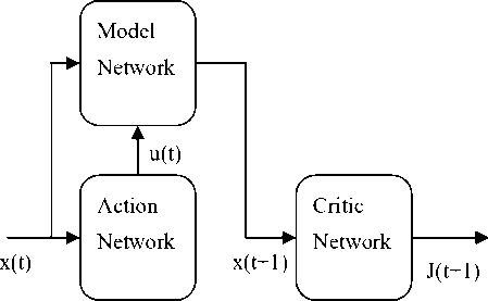
Figure 1. The basic structure diagram for ACD.

In ACD , action network and critic network are trained together, so that the two network weights can be adjusted to suit the control system to make the appropriate control decision. The output of critic network can choose cost-to-go function J or the derivative of cost-to-go function to the system parameters d J ( t )/d R ( t ) . ACD adapts heuristic cost-to-go function (J) through its own critic network. In the action dependent versions, action network is directly connected to the critic network without using models. In this paper, ADACD is used to study the optimal control of sugar crystallization.

Ш . Precalciner Kiln System

Precalciner kiln system is mainly composed of four parts, i.e., preheater, calciner furnace, rotary kiln and grate cooler. Fig. 2 is the simplified schematic of PCK system. It is characterized by the addition of a calciner furnace between the suspension preheater and the rotary kiln, in which the fuel burning exothermic process with the raw materials of carbonate decomposition process absorbing heat react extremely fast in the state of suspension or stream [7,8]. After a whirl air multi-stage preheater, raw material powder is heated. Thermal material is decomposed by the furnace, with the air flowing into the end of the preheater. After gas-solid separation, the decomposed powder flows into the rotary kiln. At this point, the rate of decomposition of material powder in the general is about 90%. With the gas coming from the bottom up, the heat that breaks down the raw materials is provided by the coal burning stove. One part of the calciner requires air coming from the exhaust gas of grate cooler. This air is named tertiary-air, with a temperature range of about 700 °C ~ 850 °C. Another part of the air comes from the gas of chamber in the back-end of kiln. Pre-decomposed raw materials follow into the kiln. Because of kiln-place tilt and rotation, materials constantly move to the head of the kiln. In the kiln, the material was heated into clinker by the reverse flowed high-temperature gas. Finally, the clinker falls into the bottom of the grate cooler through the hood of kiln, and then unloads into storage by air cooling. The airs for rotary kiln combustion come from the first-air and the secondary-air [9].

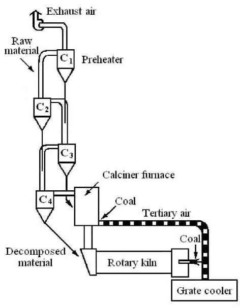
Figure 2. The simplified schematic of PCK system.

• A.    The characters of PCK System

Cement production is a complex industrial process involving mass transfer, heat transfer and physical chemistry reaction, and its stability of the production directly impacts the quality of cement. From the foregoing analysis of this paper, it can be seen that cement clinker calcination system has several notable features as follows:

• (1)    Complex physical and chemical process: The production should go through the process of combustion reaction, heat transfer of materials, water evaporation,

chemical decomposition of water, the decomposition of carbonate, the decomposition and compound of the oxide, solid-state reaction, and liquid-phase reaction, etc. Its basis theory consists of thermodynamics, dynamics, heat transfer, fluid dynamics and the crystallization of the mineralogy, and so on.

• (2)    Impact of many factors: There are many factors in the calciner process of cement production. From the perspective of process control a precalciner kiln can be seen as such a system: certain parameters of raw materials and operation act on the parameters of the device (collectively referred to as process parameters), resulting in the corresponding parameters of state. The parameters of the total number can be as many as several dozens, with functional relationship expressed as: ( Raw materials , operating , equipment )( State )

→ ( Indication )

• (3)    High non-linearity: When running at stability PCK system is in a dynamic balance as a whole. The impact of each parameter maintains a balance in this process. The changes are all non-linear in the process of running, which further increased the level of non-linearity of the system.

• (4)    Large lag: The total time from the raw powder being put into the suspension preheater to the cooler unloading clinker into silo, is about 30 minutes. Gas pumped from the cooler to be eliminated out of the preheater would take about 3 minutes. Only in the end of the cooler can one observe some state of the calcination. The above mentioned process indicates a large lag in the calcination process. In addition, some characteristics of clinker are obtained only by testing. Workers generally test clinker once in every 2 hours, and the testing process will take about 1 to 2 hours. According to the processes of the hybrid operation, it is necessary to take 1.2 to 3.2 hours to get most of characteristics of the clinker.

• (5)    Large interference exists in data acquisition: Because of the impact of the device, environment, measurement and man-made factors, collecting raw data from the process of industrial production is vulnerable to interference by noise, negligence and missing data points. The mass of raw data is often incomplete, with noise (including error or existing isolated points which deviated from the desired values) and the lack of consistency.

• B.    The balance of PCK system

In order to ensure the quality of cement, we need to pursuit three balances of the production process:

• (1)    Material balance: Raw materials heated by suspension preheater, are send into the calciner. The rate of decomposition of carbonate in the furnace gets up to 85% -95%. It is hoped that materials stay at a certain level in the process of production in reality.

• (2)    Gas balance: The direction of gas flow is in the opposite direction of materials and exhaust from the upper part of the preheater. The gas sucked in furnace and kiln relies on negative air pressure, which can be adjusted by control valve. The first-air is sucked in furnace or kiln with the coal.

• (3)    Heat balance: The needed fuel of the whole system is poured about 60% into the furnace and 40% into the rotary kiln. Heat consumption of unit clinker is dropped to below 3000kJ/kg and the thermal efficiency is raised to above 60%.

• C.    Main element analysis of PCK system

The selection of control and state variables are based on quality assurance of cement clinker under the mentioned premise. According to our analysis, the entire system should be considered to select these variables. Only a link for the single point of control to ensure the quality of clinker is meaningless. Therefore, we have adopted the following principles:

• (1)    The variables we selected should be measured directly or indirectly.

• (2)    Select the variables of normal operation of the production to make the production process more stable. Under the unusual circumstances, such as testing, kiln drying, firing, kiln hanging skin, heading, and stopping the kiln, we should use manual control.

• (3)    Select several major factors as the objects for simulation study. This is to make sure that system stability depends on major factors and to avoid non-major factors changing to major factors.

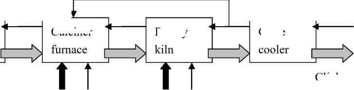
We simplify the system, and the model is shown in Fig. 3. The gray arrows indicate the flow of materials, slim black arrows indicate the flow of the air, and bold arrows indicate the flow of coal. As can be seen from the chart, the major factors which impact the system are the air and coal. Therefore, the selected variables for control are focused on air, coal, and materials. According to the analysis of the preceding sections we select state variables as follows. Among them, furnace export is a meeting point of PCK system, which reflects a number of integrated indicators for the system state. As a result, we select the temperature of the furnace export as a state variable in this article. Oxygen content of exhaust gases can indicates the extent of calcine. Lack of oxygen means materials being not fully calcined. Excessive oxygencontaining indicates excessive ventilation, which increases heat loss. Moderate oxygen assures full calcine and at the same time avoiding excessive heat loss. Therefore, this paper selects oxygen content gas of cyclone export as another state variable. Keeping theses two state variables within a reasonable range (see the under section of the definition of utility function) is the goal of production.

Tertiary-air

C 1

Pre-

heater

Grate

Calciner

Rotary

Clinker

Figure 3. Operation state of PCK system.

• D.    The neural network model of PCK system

Artificial neural network (ANN) modeling of the system is shown in Fig. 4. BP-based neural network model can better describe the non-linear system performance, and has a capacity of generalization. In Fig. 4, u_i ( t ), i = 1,2, K ,5 are the control variables of the system, including raw materials, coal-fed for furnace, coal-fed for kiln, rotary speed of kiln and negative pressure of C1 export. Variables x_j ( t ), j = 1,2 , are the temperatures of furnace export and oxygen content of exhaust, respectively.

Modeling data used are as shown in Tab. 1, which are real-time data from a new dry-process cement plant 5000t/d production line of Guigang City, in Guangxi province. Sampling time is 2 minutes. The scope of the sample data is showed in Tab. 2.

Using newff function of MATLAB neural network toolbox to set up the model, the number of network hidden layer is selected to be 60; for the hidden layer and output layer the tansig function is used. The training

u 1 (t) ________________J	The model of PCK system based on ANN	x 1 (t+1)
u2(t) ________________J
u 3 (t) ________________J
		x 2 (t+1)
u 4 (t) ________________J
u 5 (t) ________________J
x1(t) ________________J
x 2 (t) ________________J

Figure 4. Simplified model of PCK system based on the ANN.

method for model uses Bayesian normalized algorithm (trainbr). Training data are shown in Tab. 1. In Tab1, 4000 groups of data are adopted to train, 100 new groups of data are used to test the neural network model generalization ability. Training parameters are as follows:

Selection of the relevant parameters is based on

TABLE II.

R eal - time data of PCK system 5000 t / d production line

Time step	Raw material u 1 (t/h)	Coal-fed for furnace u 2 (t/h)	Coal-fed for kiln u 3 (t/h)	Rotary speed of kiln u 4 (r/m)	Negative pressure of C1 export u 5 (kPa)	Temperature of furnace export X 1 ( ^ )	Oxygen content of exhaust x 2 (%)
t	444.411	18.992	15.06	3.72	-5.322	880.13	3.192
t+1	452.079	17.869	15.06	3.775	-5.322	875.98	3.192
t+2	453.394	19.748	15.06	3.72	-4.974	880.37	2.448
t+3	450.296	19.748	15.06	3.765	-4.974	886.47	2.448
t+4	426.181	19.748	15.06	3.724	-4.974	880.62	3.076
t+5	457.431	19.748	15.06	3.769	-4.974	881.35	3.076
t+6	452.896	19.748	15.06	3.726	-4.974	880.13	3.076
t+7	384.061	19.748	15.06	3.738	-5.2315	883.79	3.076
t+8	426.334	19.748	14.555	3.739	-5.492	885.25	3.076
t+9	438.636	19.748	14.555	3.726	-5.492	892.09	2.551
t+10	460.798	18.18	14.555	3.767	-5.492	902.34	2.551
t+11	463.161	17.615	15.06	3.723	-5.492	902.59	2.551
t+12	427.905	17.615	15.06	3.765	-5.492	883.54	3.241
t+13	469.256	18.427	15.06	3.731	-5.492	871.09	3.241
t+14	462.443	19.005	14.55	3.765	-5.322	866.46	3.241
t+15	421.268	19.005	14.55	3.724	-5.322	871.83	3.241
t+16	439.972	19.005	14.55	3.77	-5.322	883.54	6.482
t+17	437.313	18.415	14.55	3.715	-5.322	886.72	2.905
t+18	445.191	18.415	14.55	3.746	-5.322	881.1	2.905
t+19	442.332	18.979	14.774	3.735	-5.322	877.93	2.905
t+20	456.441	18.979	14.774	3.736	-5.322	880.13	2.905
......	......	......	......	......	......	......	......

TABLE I.

T he scope of sampling data

Data scope	Raw material u 1 (t/h)	Coal-fed for furnace u 2 (t/h)	Coal-fed for kiln u 3 (t/h)	Rotary speed of kiln u 4 (r/m)	Negative pressure of C1 export u 5 (kPa)	Temperature of furnace export X 1 ( ^ )	Oxygen content of exhaust x 2 (%)
max	488.176	22.128	15.908	3.992	-4.82	967.04	8.557
min	360.727	6.506	14.111	1.935	-5.7705	847.66	1.678

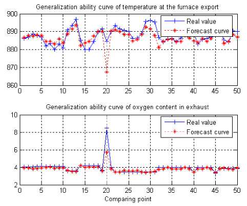
Figure 5. Fitting curve of PCK system model after training.

W . ADACD Controller Design for PCK System

• A.    The principle of ADACD

A typical ACD consists of the three networks: Critic Network, Model Network and the Action Network. ADACD is an Action-dependent form of ACD. ADACD includes: Critic Network and the Action Network, which combines Critic Network and Model Network to form a new Critic Network [10]. The new Critic Network in fact implies a model, but also refers to the output/ implementation u of Action Network. This simplifies the structure of the system and increases the flexibility of the method in the application, so as to avoid building accurate system model, which might not be easily obtained in practice.

In action dependent ACD, action is directly connected to the critic without using models, including action network and critic network, as shown in Fig 6. The Action Network is the traditional sense of controller. The critic network is separated from the action network. When the critic Network and the action Network are separated, it is possible to have more ways to adjust and strengthen the controller for learning.

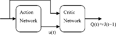
Figure 6. Schematic Diagram of ADACD.

is the key of Adaptive Critic Design methods for training and learning.

According to equation (6), for all the t, when E c ( t ) = 0 , we can further deduce:

Q ( t ) = U ( t + 1) + y Q ( t + 1)

= U ( t + 1) + y [ Q ( t + 1) + yQ ( t + 2)]

= •••                                           (7)

»

= £ Y - ' ^{- 1}U ( k )

k = t + 1

• B.    The critic and action network training for ADACD

In ADACD methods, the output of Critic Network is cost function Q ( t ) . Assuming achieving the training of network by minimizing the following error function:

• e . ( t ) = £ |u Q ( t ) - Q ( t - 1) + U ( t )]² (6) t 2

where Q ( t ) = Q [ X ( t ) , u ( t ) , t ] , U ( t ) is the moment of t's utility function, Y ( 0 <  Y <  1 ) is the discount factor. In general practice, the cost function of Q ( • ) needs to be evaluated by Critic Network, U ( • ) is the basic utility function which is given by the practical issues. We can get the evaluation of U ( t ) by Critic Network's twice continues outputs Q ( t ) and Q ( t + 1) . We compare the difference between estimated value and expected value, to get the needed error sequence, whose squares are seen as the object function of the optimization process [11]. The definition of utility function in advance

ADACD has only action network and critic network. In this Fig 6, the action network outputs the control signal u ( t ) , and the critic network outputs an estimate of cost function Q ( t ) . Fig.7 is the schematic diagram for implementation of our proposed ADACD controller. The solid lines represent signal flow, while the dashed lines are the paths for parameter tuning of the critic network and the action network. It will generate control signal u ( t ) when the action network accepts the system state x ( t ) , then u ( t ) and x ( t ) add to the critic network which will output an approximate of Q function (equation (7)). In Fig.7, PCK system is the neural network model for the cement factory as discussed in the fourth section, which accepts the control signal u ( t ) from the action network outputs and generates the new state X ( t + 1) . In addition, U ( t ) is the utility function, and Y is the discount factor and Z ¹ is the time-delay operator [12].

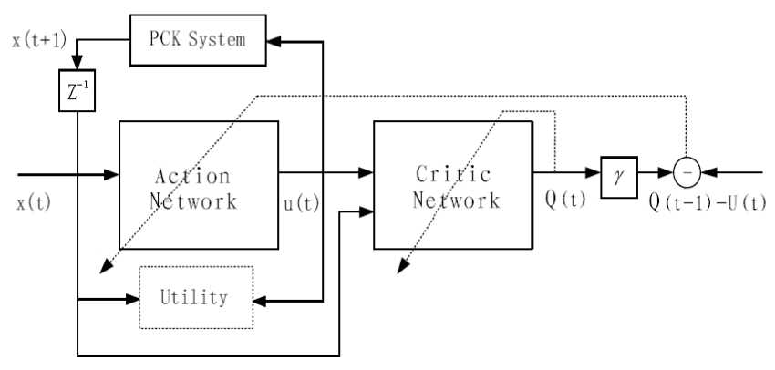
Figure 7. Schematic diagram for implementations of ADACD Controller

For the critic network, whose output is Q(t) , the weight update needs an error between the real output and the desired output of the critic NN. The training for network has two phases: the forward computation process of the network and the errors back-propagation process to update the weights of the network. Critic Network's outputs are used to approximate Q(t) of equation (7), and the aim for training Critic Network is to minimize the error function as follow:

e c ( t ) = Q ( t ) - Y • Q ( t + 1) - U ( t )]         (8)

1      9

E c ( t) = 2 • e c ²( t )

The weight update rule for the network is gradient descent rule, which is given by the following equations:

w_c ( t + 1) = w c ( t ) + A w c ( t )

^A w c ⁽ t ) = l c •

-

) i (jEE® ^ ^ 5 W c ( t ) J c I 5 Q ( t ) d W c ( t ) J

where l_c is the learning rate of the critic network, and у is the discount factor and W c is the weight vector in the critic network. For the critic network, the hidden layer uses the sigmoidal function given by:

The critic network is chosen as a 7-10-2 structure with 7 input neutrons, 10 hidden layer neutrons and 2 output neutrons. The 7 inputs are 2 states (the temperature of the furnace export and the oxygen content of exhaust) and 5 control variables. These control variables represent raw materials, coal-fed for the furnace, coal-fed for kiln, rotary speed of kiln and negative pressure of C1 export, respectively. The structure of the action network is chosen as 2-10-5 with 2 input neutrons, 10 hidden layer neutrons and 5 output neutrons. The 2 inputs are the 2 state variables, and the 5 outputs come from the 5 control variables, respectively. Based on the analysis of the data from the field, and The “three required balances” discussed in section 3, we can concluded that if the temperature of the furnace export can be controlled at around 850-930 ^ , and the oxygen content of exhaust is in the control of 2% to 4% within the scope of the changes, the requirements of the production can be met. The utility function is defined as:

U(t) =

0, (x1 (t) - 890 < 40) U (x2 (t) - 3| < 2)1, others

У =

1 - e

1 + e -^x

In the MATLAB environment, it can easily call tansig function to achieve (12). The output layers adopt linear function.

The main objective of action network (action NN) is to generate a sequence control signal u(t) to make the performance index be optimal.. The aim of training the action network is minimizing the output of the critic network Q ( t ) , and the weights updating equations in the action network are as follows:

e a ( t ) = Q ( t ) (13)

E a ( t ) = 2 • e 2 ( t )                     (14)

where X j ( t ), j = 1,2 , are the temperature of the furnace export and the oxygen content of exhaust, respectively.

The simulation experiments have been shown in Fig. 8 and 9. Multiple experiments show that, in spite of the random initialized weights of neural network, the controller can control the state variables in the required scope. From Fig.8, we can see after the small fluctuations at the beginning, the temperature of furnace export and the oxygen content of exhaust tend to stabilize, and their fluctuations are within the scope of the utility function defined in (17). Fig. 9(a) shows the coal changes of fuel feeding system. Fig. 9(b) shows raw materials feed, rotary speed, C1 negative changes in the export. Those changes of Fig. 9 are similar to the change in temperature trends in Fig. 8, which is being stabilized step-by-step after a period of fluctuations.

^Wa ⁽ t ⁺ 1) = ^Wa ⁽ t ) ^{+ A W}a ⁽ t )

^A w a ⁽ t ) = ^la •

V

d E a ( t ) t 5 w a ⁽ t ) J

d E a ( t ) d Q ( t ) d u ( t ) V"a Q ( t y 'mT) 'dw^Y) J

where l_a is learning rate of the action network, and w_a is the weight vector in the action network. For this network, both hidden layer and output layer use the Sigmoidal function as shown in the equation (12).

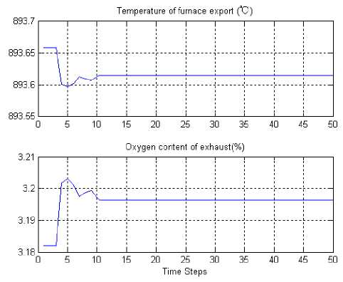
Figure 8. Result for the PCK system control.

• V . Simulation Results and Conclusion

  
  
  

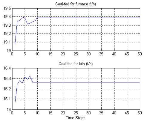
  Figure 9(a). Control variables changed curve for coal.

  
  
  

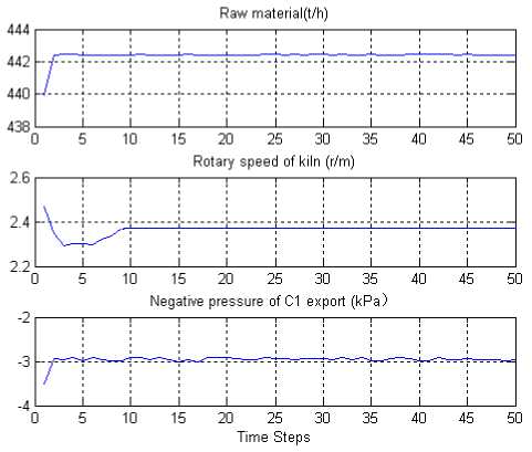
Figure 9(b). Control variables changed curve for raw materials, rotary speed of kiln and negative pressure of C1 export.

In this paper, the results show that the ADACD improves the system operation stability more effectively than manual operation. For a large scope of changed data, the proposed method can give a good performance on control. For such a complex system, PCK system without clear expression of their mathematical model of reality, ADACD method can achieve better control of the output of the system. However, the model of PCK system should be improved further, in order to enhance generalized ability of the model.