Adaptive Compensation of Unknown Actuator Failures for Strict-feedback Systems

Published Online August 2011 in MECS                               'll1 and Computer Science у ркея

Actuator failures seem inevitable in practice especially in complex systems. The unknown failure may cause instability and catastrophic accidents during operation of control systems. As we all know such failures are often uncertain in time, value and pattern, namely it is not known when, how much and how many actuator fail. So it is difficult to address the problem of actuator failure compensation. To address such problem, serval different design methods have been proposed such as multiplemodel designs and switching and tuning techniques, fault detection and diagnosis-based designs, robust control designs, neural network techniques, sliding model method. It is well known that adaptive control systems can obtain desired performance by adjusting controller parameters with system response errors during the operation of control system. So compared with other methods, It avoid false alarms and delays caused by failure detection.

In the context of adaptive control, several schemes based on adaptive control approaches have been proposed, see for examples in [1]-[7] and [10]-[12]. In [1] [2], adaptive controller were proposed to linear systems with parameter uncertainties. It was extended to nonlinear systems in [3] with backstepping techniques to guarantee

Manuscript received January 1, 2008; revised June 1, 2008; accepted July 1, 2008.

Copyright credit, project number, corresponding author, etc.

stability and tracking performance of closed-loop system. The results had been extended to MIMO systems with unknown actuator failures In [5]. An output feedback control law was designed for strict-feedback nonlinear systems with backstepping techniques to compensate unknown actuator failures in [4]. In [6] an adaptive output feedback control law was proposed to linear systems. It was expended to the nonlinear systems with in [7]. A state feed-back control law was proposed to compensate unknown failures and guarantee transient performance in [11]. In [10] the problem of compensation of hysteric actuator failures had been discussed.

The work of this paper aim at compensating unknown actuator failures for a class of nonlinear systems with unknown constant parameters and bounded external disturbance. Several different actuator failure patterns are considered including partial loss of effectiveness, total loss of effectiveness as shown in [6]. Note that total loss of effectiveness denotes the output of actuator is fixed on an unknown constant no matter how much is the input. So the uncertainties caused by the failure of total loss can be seen as the bounded disturbance. A state feedback control scheme is proposed by using backstepping techniques. Compared with exist results about compensation of unknown actuator failures, we design an estimator to estimate the upper bound of uncertain term caused by the failure of total loss. The stability of closed-loop system and output tracking performance can be ensured by our control law and corresponding update laws of uncertain parameters.

The remaining part of this paper is organized as follows. In section 2, the control plants are given and the mathematical model of actuator failures are discussed. In section 3, control scheme is proposed. Then we give the stability analysis. Simulations results given in section 4 on a practical systems and it confirm the control scheme are effective.

• II.    problem statement

We consider a class of nonlinear systems with uncertain parameters and m inputs. The system model is given as

Х 1 = x 2 + У ^т ф 1 (x 1 ) x₂ = x 3 + У ^т ф ₂(x 1 , x 2 ) :                                                   (1)

^x n = ^Ф п ⁽ x ) ' Z b" ⁺ d ⁽ t )

=1

y = x ₁

where x = (x1,x2,•■■,xn) is system state, y = x1 e R is output of system and ф. e Rp (г = 1,2, — , n) are known continuous function. bj (j = 1,2, —, m) e R and У e RP are unknown constant parameters. ui(i = 1,2, — ,m) are inputs of the system. d(t) is unknown external disturbance.

We now consider the adaptive compensation control of system (1) for the following actuator failure problem. As shown in [7], the mathematical model of the failure of th actuator at time instant t f can be modeled as u =σ v +u ,(∀t≥t f) σ u =0

where 0 ≤ σ ≤ 1, u and t _f are unknown constants. It is clear that the actuator works normally namely u = v denotes the constant σ = 1 . Other cases are discussed as follows

1 ， 0 < σ < 1

It indicates u = σ v . The th actuator is called partial loss of effectiveness.

2 ， σ = 0

It indicates u = u . The th actuator is called total loss of effectiveness.

With above mathematical model of actuator failures, system (1) can be rewritten as follows x1 = x 2 + S ф1( x1)

x ₂ = x 3 + Уф 2 ( x 1 , x ₂)

:                                                          (3)

x n = ^{у т} Ф п ( x ) + e b ^ v + e bu + d ( t )

=1               =1

y = x ₁

The following assumptions are necessary to design adaptive controller

Assumption 1: System (1) is such that for any up number m - 1 of total failure actuators, the remaining actuators can still achieve the desire control objectives. Any actuator changes only from normal case to one of the failure case.

Assumption 2: b ≠ 0 , the sign of b is known.

Without loss of generality, we suppose s gn ( b ) = 1.

Assumption 3: Reference signal y_r ( t ) and its -order ( i = 1,2, — , n - 1) derivatives are known and bounded.

Our purpose is to design control scheme to guarantee globally stability of closed loop system.

Ш . DESIGN OF ADAPTIVE CONTROLLERS

Before propose the adaptive control scheme, to using backstepping technology as in [8] [9], the following coordinates transformations are introduced.

z1= x1- yr z t = x- - a--1 - y(-1),(i = 2, —, n)

where z 1 is the tracking error and a_{i - 1} (i = 2,3, — , n ) is the virtual control in step .

Step 1: With (3) and (4) we can get

• •                 ••

z ₁ = x ₁ - y_r

= x2 + ^ф1(x1) - yr(5)

= z ₂ + α ₁ + θ ^T ϕ ₁( x ₁)

where α ₁ is the virtual control. The following Lyapunov function is considered

V =1 z 2 +1У T r-1<9(6)

where У = 9 - У , У is the estimation of У and Г is a positive define matrix.

Virtual control α ₁ can be chosen as

α ₁ =- c ₁ z ₁ - θ ˆ ^T ϕ ₁( x ₁)                        (7)

where c ₁ is positive constant. With (5) (6) and (7), the derivative of V ₁ is

• V 1 = z 1 z 1 - У T Г - ¹(У

= z 1 ( z ₂ + a 1 + Уф 1 ( x 1 )) - У T Г -1 У

= z 1 ( z ₂ - c 1 z 1 - У T (p_x ( x 1 ) + S T ф 1 ( x 1 )) - У T Г -1 У    (8)

= z 1 z ₂ - c 1 z 1² + У T ф_х ( x 1 ) z 1 - У T Г -1 У

= z 1 z ₂ - c 1 z 1² - У T Г^{- 1} ( У - T 1 )

Turning function can be chosen as

τ ₁ = Γ ϕ ₁ z ₁                       (9)

Step 2: With coordinates transformations (4) and system model, we can get the derivative of z ₂ as follows (2) z ₂ = x ₂ - α ₁ - y_r ⁽²⁾

= x 3 + θ ^T ϕ 2 ( x 1 , x 2 ) -^{∂ α 1} ( x 2 + θ ^T ϕ 1 ) -^{∂ α 1} θ ˆ

3212 _∂ x ₁ 21 _{∂ θ}

∂ α

¹ y r ∂ y_r

- y r ⁽²⁾

= z ₃ + α ₂ + θ ^T ϕ ₂( x ₁, x ₂) - ^{α 1} ( x ₂ + θ ^T ϕ ₁)

∂ x ₁

да &  da .

-1θ-1yr ∂θ    ∂yr where α2 is the virtual control in this step. The following

Lyapunov function is considered

V 2 = V 1 + ¹ ₂ z 2²                         (11)

Virtual control α ₂ can be chosen as

T α ₂ =- c ₂ z ₂ - z ₁ - θ ^T ( ϕ ₂

∂ α ₁

∂ α ₁

-

∂ x ₁

∂ x ₁

∂α∂α

+ ¹ τ ₂ + ¹ y_r

∂θ    ∂yr

where c ₂ is positive constant. With (5) (6) and (7), the derivative of V ₂ is e                  e

2 z 2

= z_i z 2 - c z 2 - 9 ^T Г ^ 9 - t ₁ ) + z ₂ ( z 3 + 9^T Ф 2 ( x_i , x 2 )

+ «2 - — (x 2 + 9 Ф^ -   9 - — yr)

∂x1              ∂θ    ∂yr

2 T -1                              T

= z ₁ z ₂ - c ₁ z ₁ ² - θ ^T Γ ¹ ( θ - τ ₁) + z ₂( z ₃ + θ ^T ϕ ₂( x ₁, x ₂)

-

c ₂ z ₂

-

T    ∂α∂α∂α z1-θT(ϕ2-1ϕ1)+1x2+1τ2 ∂x1∂x1∂θ

+ ¹ y r - ¹ ( x 2 +θ ^T ϕ 1 ) - ¹ θ- ¹ y r )

^∂ y r      ^∂ x 1               ∂θ

∂ y_r

r

r

e

= - c _i z 2 - c ₂ z 2 + z ₂ z 3 - 9 ^T r^{- i} ( 9 - t ₁ )

-

T    ∂α

+ θ ^T ( ϕ ₂ - ¹ ϕ ₁) z ₂ ∂ x ₁

22 =- c ₁ z ₁ - c ₂ z ₂ + z ₂ z ₃

-

d o-⁹ — т 2 ) z 2

∂ θ

- θ ^T Γ^{- 1} ( θ - τ ₂)

Turning function can be chosen as ∂ α τ ₂ = τ ₁ +Γ ( ϕ ₂ - ¹ ϕ ₁) z ₂ ∂ x ₁

^^ ^{- т} 2 ) ^z 2 ∂ θ

Step (ii = 3,---,n -1): The same as analysis above, the derivative of zi is zi

= x_i - α _{i - 1}

- y r ^{( i )}

= x+i + 9Ф((xi,x2 L,x)- dii-i - уГ()

= z_{i +} i + 9ф ( ( X i , x 2 l , x ) - (X i - i + a

-1 _∂ α

= z i +i ⁺ ^Ф ( ⁽ x i , ^x 2 L ,x i ) ^- E^ - k =1 ∂ x k

• ^- ∂ α ∂ α

• -1 y k _-    - 1 _{θ +} α

∑ _{k = 1 ∂} y_r k -1 r _{∂ θ} ˆ

( x_{k + 1} + θ ^T ϕ _k )

-

-

Considering the following Lyapunov function

V = V + ¹ z ²

-1

The virtual control in this step can be designed as follows

- ∂α

-1 -θT (ϕ -∑   -1ϕk)

k =1 ∂ x k

-1 _∂ α

+ ∑ ^- k =1 ∂ x k

₊ -1 _∂ α _{k -}

^∑ k =2 ∂ θ ˆ

-∂α∂α xk+1 +∑k --11yrk +    -1τ

k=1∂yr        ∂θ

-1

1Γ(ϕ -∑   -1ϕl)zk l=1 ∂xl where c is positive constant. We can get the derivative of V is as follows

Vi = V 1+ z, z,

-1

• V -1	/         d a _i k  да_л & + z ( z + 1 - ∑    k - - 1 1 yr k -    - 1 θ + α k =1 ∂ y rk 1        ∂ θ
-1 ∂ α + 9 Т Ф ( x i , x 2 L , x i )  E 'i ( x k +i + 9Ф к )) k =1 ∂ x k
•	,      da . &  da .
V -1	+ z ( z - - 1 θ ˆ + - 1 τ - cz - z +1 ∂ θ ˆ ∂ θ ˆ               -1

-1 _∂ α

^{- 9 (} Ф ^- Е ^^ Ф k ) ^{+ 9} Ф (⁽ X i , X 2 L ,X i ) k =1 ∂ x k

+∑i1∂αk-1Γ(ϕ -∑i1∂α k=2 ∂θ          l=1 ∂xl

-1∂α ϕl)zk-∑ k=1 ∂xk

-1 _θ T

^ϕ k )

k =1

• ■V - da_k - i &

• - ∑ z_k    ^{k 1} ( θ - τ )

k =2     ∂ θ

Turning function is

• ^- ∂ α

τ =τ -1+ Γ(ϕ -∑    1ϕk)z

∂x k=1     k

zn

Step n : From (3) and (4), we can get the derivative of is as follows yr(n)

m

• •                  •                  •

z=x-α - nnn-1

= θ ^T ϕ _n ( x ) + ∑ b σ v

m

= θ ^T ϕ _n ( x ) + ∑ b σ v

m

-

y_r ( n )

m                  n -1

∑ b u + d ( t ) - ∑ ^{∂ α} k ⁿ - ^- 1¹ y r^k

=1                  k=1 ∂yr n-1

• - ∑    ^{n - 1} ( x k +1 + θ ^T ϕ k )

k =1 ∂ x k

-

^{d a} n .L 9 - y ( ⁿ ) ∂ θ      ^r

Because u represents the actuator’s output when actuator is total loss of effectiveness . According to the mathematical model of th actuator, we can get u and b

m are unknown constants. It is clear ∑b u is unknown

=1

m constant and bounded. Let d(t)=∑b u +d(t)and itcan =1

be seen as the bounded external disturbance term. then (20) can be rewritten as

m

n -1

-∑   n-1 (xk+1 +θTϕk) - k=1 ∂xk

n -1 _∂ α _{n - 1 k}

• ^- ∑ _∂ k -1 y r

^{k = 1 ∂ y r}            (21)

^da n -i &  _v( n )

θ - y

∂θ     r

If knowing the system parameters and failures, the control input v can be chosen as

vi=ρα

1 ρ = _m ∑ σ _i | b_i | i =1

where α is the virtual control in the last step and will be

m given later. According to Assumption 1, ∑σi|bi|> 0 is i=1

unknown constant owing to the unknown actuator failures and unknown system parameters. So we must replace the unknown ρ with its estimate ρ ˆ in the control law (22) and the controller is designed as

Control law:

v_i = ρ ˆ α

The virtual control α is designed as n-1

α = - z_{n - 1} - c_nz_n - sign ( z_n ) D ˆ - θ ˆ ^T ( ϕ _n - ∑    ^{n - 1} ϕ _k )

k =1 ∂ x k

n -1                                         m

V = ^- E cP ^{+ z}„ -1 ^z„ ^{+ z}„ P T Ф„ ( x ) ⁺ E b ^CT ( Р ^- p ) «

-

n -1                   n -1

∑ _k ⁿ _- ^- ₁ ¹ y r^k - ∑ ^{n - 1} ( x k +1 + θ ^T ϕ k ) - y r ^{( n )} + d ( t ) k =1 ∂ y r         k =1 ∂ x k

∂αn-1 ∂θ n-1

-∑zk k=2

- 9 - ^- d D - ¹ m b a , ^ - 9 ^т Г^{- 1} (9 - T n -1 ) ηγ i =1

a-- «? - t ,)

_{∂ θ} ˆ        n -1

n -1                                              m

= -E czi + zn-1 zn + zn (PФп (x) + a -E bCTPP i=1                                                                   i=1

-

n -1                   n -1

∑ ^{n - 1} y_r ^k - ∑ ^{n - 1} ( x_{k + 1} + θ ^T ϕ _k ) - y_r ^{( n )} + d ( t ) k =1 ∂ y r^{k 1} k =1 ∂ x k

+ ∑n-1∂αn-∑k=1 ∂xk +n-1∂αk- k=2 ∂θ

n -1 _∂ α _{n - 1} x k +1 ∑ _{k = 1 ∂} y_r k -1 Γ ( ϕ n - ∑ ^{n - 1 ∂ α n -} l =1 ∂ x l

y ^k + ^{∂ α n - 1} τ + y ⁽ r _{∂ θ} ˆ nr

ϕ _l ) z_k

-∂αn-1 ∂θˆ n -1

- ∑ z k k =2

.9^ - 1 Df ) - ¹ E b i CT i pp - 9 ^T r^{- 1} (( 9 - T n -1 ) ηγ =1

^d f k r¹ (^^ ^- T n -1 )

∂ θ

where a ˆ , D ^ˆ are estimation of unknown constant a and D . D is the upper bound of d ( t ). τ _n is the turning function in this step and can be chosen as follows

With the virtual control α given in (24), the derivative of Lyapunov function can be re-written as n -1

V =- ∑ c z ² + z_{n - 1} z_n + z_n ( θ ^T ϕ _n ( x ) - z =1

- cz nn

n - 1 _∂ α τ _n = τ _{n - 1} +Γ ( ϕ _n - ∑    ^{n - 1} ϕ _k ) z

∂x k=1     k

Update laws:

θ ˆ = τ _n

D=η|zn | ρˆ = -γαzn where Γ is a positive define matrix and η and positive constants.

We consider the following Lyapunov function

m

V = V i+¹ Zn ² +— d ² +— Е b стр ² n -1 2 n 2 η 2 γ ∑ _{i = 1} ii

The derivative of V is

m

V = V n -1 + Z , z , - 9Г ^{- 1} 9 - -DD - - E I b |

ηγ i =1

n -1 _∂ α

- s gn ( z_n ) D ^ˆ - θ ^{ˆ T} ( ϕ _n - ∑ ^{n - 1} ϕ _k ) + d ( t ) k =1 ∂ x k

∂ α n - 1 τ ₊ y

∂θ n

m

+∑n-1∂αn-k=1  ∂xk n-1 ∂αk

γ are

-

k =2 ∂ θ ˆ n -1 _∂ α _{n - 1} ^∑ k =1 ∂ y r^{k - 1}

- ∂αn-1 ∂θˆ n-1

^- ∑ z k k =2

n -1

=- ∑ c_iz_i ² + z_{n - 1} z_n + z_n ( θ ^T ϕ _n ( x ) + ∑ b_i σ _iv_i + d ( t )

-

n -1                   n -1

∑ ^{∂ α n - 1} y r^k - ∑ ^{∂ α n - 1} ( x k +1 + θ ^T ϕ k ) - y r ⁽ k =1 ∂ y r^{k 1}        k =1 ∂ x k

a1- 9 - 1 DD - 1 Eib | oipb

∂θ     η γi=1

With (22) and (23), the derivative can be rewritten as follows

n -1 _∂ α _{n - 1} x k +1 ∑ _{k = 1 ∂} y_r k -1

1Γ(ϕn- ∑n-1∂αn- l=1 ∂xl

k

r

Ф/) zk -E bp pp

=1

n -1

y r^k - ∑ ^{∂ α n - 1} ( x k +1 + θ ^T ϕ k ) - y r ^{( n )} k =1 ∂ x k

m

- 9^ ) - - E bp, pp - 9 T r^{- 1} (^? - T n -1 ) γ =1

^{d a} k e¹ ( 9 ) - T „_ 1) -¹ DDD

∂θ      n1 η

=- ∑ c z ² + z_{n - 1} z_n + z_n ( θ ^T ϕ _n ( x ) - z_{n - 1} - c_nz_n =1

n -1

- s gn ( z_n ) D ^ˆ - θ ^{ˆ T} ( ϕ _n - ∑ ^{n - 1} ϕ _k ) + d ( t ) k =1 ∂ x k

∂ α _{n -}∂ θ ^ˆ

m

n-1 ∂α τn+∑k- k=2 ∂θ

n -1 _∂ α Γ ( ϕ n - ∑

∂ x_l

^∂ α n - _ˆ

n -1

ϕ _l ) z_k

n -1

• -E b.CTa p - E -p-19 тФк-k=1 ∂xk

m

• 1E b,CT, pp - 9т Г-1(9 - Tn-1)

γ =1

-

DD

-

•

∂ θ

•

ˆ

θ ˆ)

η n-1

- ∑ z k k =2

dak-r(9 - Tn-1) ∂θ

Further simplification, we can get

n -1

V =- ∑ c_iz_i ² + z_{n - 1} z_n + z_n ( - z_{n - 1} - c_nz_n - sign ( z_n ) D i =1

n-1 +d (t)+вт (Фп-grand k=1 ∂xk ϕk)- ∂αn-1(θˆ-τn) ∂θ n-1∂α         n-1∂α +∑  k-1Γ(ϕ -∑n- k=2 ∂θ         l=1 ∂xl 1ϕl)zk m -g bp ap) =1 1          :                            : -1 DDˆ -θTΓ-1(θ-τn-1) η n-1 -∑z k=2 дak--(X-t k       (θ-τn-1) ∂θ m 1 - ∑b σ ρρ γ =1 n =-∑c z 2 +zn(d(t)-s gn( =1 n)Dˆ) - DD η n-1

• -    9ТГ-Чв - (Tn-i-Гф, -g .   фk)zn))

k =1 ∂ x k

• -    2 z k О ¹ ( в - ( T n —i +г ( Ф п - 2 Оф ,) z n )) k = 2     ∂ θ                        l = 1 ∂ x l

• 1    m^a

• ^-    2 b ^{ap (} P ⁺ Y« z n )-- n Tp- ^{( в - T} n ) z n

γ _{i = 1} ii         n    _{∂ θ}

With turning function given in (25), we can get

• -    вт гфв - Tn)-g zk O^ (в) - Tn) k=2∂

• 1    v                  ^{d a} -l & л x

—2 b p p % ⁽ p d ⁺ Y^{a z} n ) —- n- ( e ^{- T} n ) z n

γ _{= 1}                n     _{∂ θ}        n n

n

∑ c z 2+|zn|(D-Dˆ)-1DDˆ

• = 1                     η

• -    e ^т r ^{- 1}( 6 - T n ) - g z . ^ O t^ в - л ,)

k =2     ∂ θ

• -    V                 ^{d a} -i &n

  --2 b ^ i P ⁽ P ⁺ Y^{a z} n )-- -n- ^{( e - T} n ) z n

γ _{= 1}                n     _{∂ θ}        n n

n

≤- ∑ c z ²

=1

1 I

- 1 D ( D ˆ - η | z n ^η

1 ^m

• -    g b Pi P ( f D + Ya z , ) γ =1

n--   da-i zz)x

• - ∑zkk-1(θ-τn) k=2

  _-

  
  

  I |) - θ ^T Γ^{- 1} ( θ ˆ - τ n )

  
  

  a-^ ( ^ D - T n ) z , ∂ θ

  
  

With the update laws in (26), the derivative of V is

n

V≤-∑c z 2

=1

Theorem 1: Consider the nonlinear uncertain system (1) with unknown parameters, external disturbance and unknown failures which modeled by (3) of m actuators and satisfying Assumption 1-3, under the control law in (23) (24) (25)and the update laws in (26), all signals in closed loop system are bounded and the asymptotic tracking is achieved, i.e. lim( y - y_r ) = 0 .

t →∞        ^r

Proof: Based on the above analysis, signal z,, в, D, P% are bounded. Then the virtual control α and the control input v are also bounded. By applying the LaSalle-Yoshizawa theorem in (30), we can get lim z, = 0, (1,2, l, n) . So the asymptotic tracking is t→∞ achieved, i.e. lim(y- yr) = 0 . t→∞

W . SIMULATION STUDIES

In this section, we use the same valve control mechanism of a liquid tank dynamics model shown in Figs.1 as in [9]. The transfer function can be expressed as. It can be described as follows

• h ( s ) = G ( s )( b ₁ u ₁( s ) + b ₂ u ₂( s ) + d ( s ))         (31)

where h is state and denotes the height of water surface, transfer function G ( s ) = ks . k , b ₁ and b ₂ are unknown constants. d ( s ) is unknown disturbance with unknown constant upper bound. u ₁( s ), u ₂( s ) are input signals of system.

With Laplace transformation, system model (31) can be rewritten as hi = kb1 u1 (t) + kb2 u 2 (t) + kd (t)              (32)

Let b1= kb1 and b2= kb2 , d(t)= kd(t) can be seen as unknown disturbance. The model (32) can be rewritten as follows h=b1u1(t)+b2u2(t)+d(t)              (33)

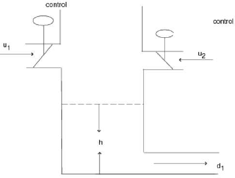
Figure.1 Valve control mechanism of a liquid tank

In simulation, the actual parameters value are k = b ₁ = b ₂ = 1 . The uncertain disturbance d ( s ) is 0.1sin( t ) .

We choose η = γ = 0.5 and feedback gain c = 20 . The initial value are chosen as follows: z ( 0 ) = 0.5, ρ ˆ(0) = 0, D (0) = 0.

Let the reference signal is y _r ( t ) = ln( t ) . Figs.2 is tracking error, Figs.3 and Figs.4 are input u ₁ ( t ) and u ₂ ( t ) supposing at t = 10 second actuator u ₁ ( t ) is stuck at an unknown value 1.5. When all actuators work normally, Figs.5 is tracking error, Figs.6 and Figs.7 are input u ₁ ( t ) and u ₂ ( t ).

Let the reference signal is y _r ( t ) = sin( t ). Figs.8 is tracking error, Figs.9 and Figs.10 are input u ₁( t ) and u ₂ ( t ) supposing at t = 10 second actuator u ₁ ( t ) is stuck at an unknown value 1.5. When all actuators work normally, Figs.11 is tracking error, Figs.12 and Figs.13 are input u ₁ ( t ) and u ₂ ( t ).

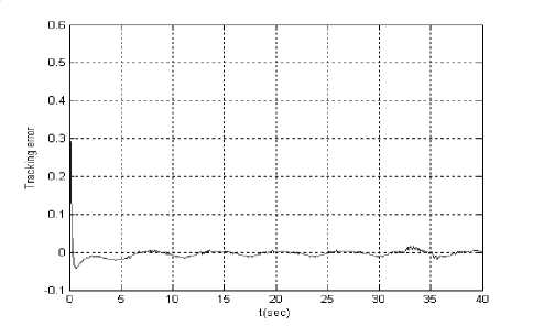
Figure.5 Tracking error ( y_r ( t ) = ln( t ) )

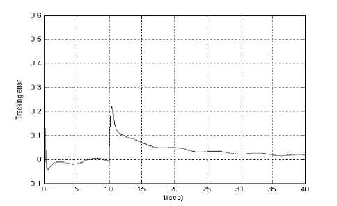
Figure.2 Tracking error ( y_r ( t ) = ln( t ) and failure)

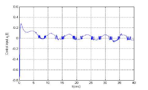
Figure.6 Input u ₁ ( t ) ( y_r ( t ) = ln( t ))

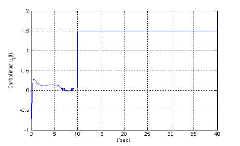
Figure.3 Input u ₁ ( t ) ( y_r ( t ) = ln( t ) and failure )

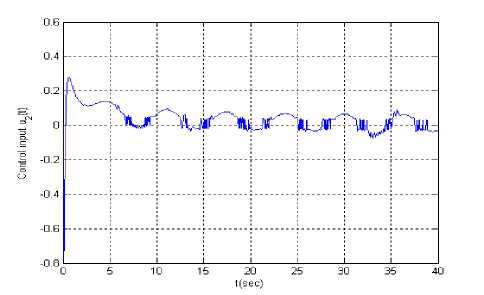
Figure.7 Input u ₂ ( t ) ( y_r ( t ) = ln( t ))

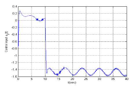
Figure.4 Input u ₂ ( t ) ( y_r ( t ) = ln( t ) and failure )

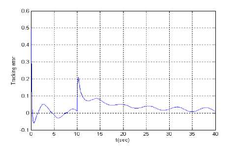
Figure.8 Tracking error ( y_r ( t ) = sin( t ) and failure)

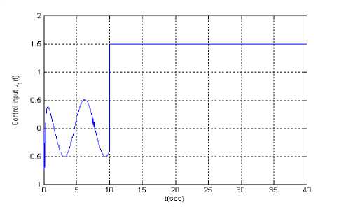
Figure.9 Input u ₁ ( t ) ( y_r ( t ) = sin( t ) and failure )

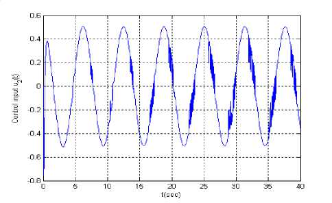
Figure.13 Input u ₂ ( t ) ( y_r ( t ) = sin( t ))

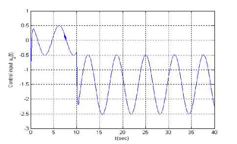
Figure.10 Input u ₂ ( t ) ( y_r ( t ) = sin( t ) and failure )

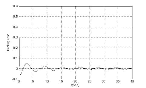
Figure.11 Tracking error ( y_r ( t ) = sin( t ))

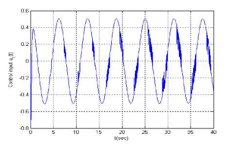
Figure.12 Input u ₁ ( t ) ( y_r ( t ) = sin( t ))

• V . CONCLUSION

An adaptive state feedback control law is proposed for a class of uncertain nonlinear systems with unknown parameters and unknown external disturbance to compensate unknown actuator failures. The uncertainties caused by unknown actuator failures are seen as the bound disturbance and handled by designing an adaptive estimator to estimate its unknown upper bound. Our control law and update laws can guarantee the stability of closed loop system and tracking performance.

A cknowledgment

This work is supported by science foundation of Zhejiang Water Conservancy And Hydropower College (xky-201102).