Addressing the Bandwidth issue in End-to-End Header Compression over IPv6 Tunneling Mechanism

Published Online August 2015 in MECS DOI: 10.5815/ijcnis.2015.09.05

• I.    Introduction

  Internet is growing at an alarming rate and with the advent of new devices and applications it’s not possible to sustain with the IPv4 internet protocol. IPv4 is a 32 bits addressing protocol [1], which can address up to 232 devices. But the internet users are much more than this number. So, the need of a new addressing protocol was felt in 1998 by IETF, and this is known as the next generation internet protocol IPv6 [2], which is a 128 bits protocol which can address up to 2128 devices, such a huge number. It means each and every particle on the earth will be addressed; still we are left with a huge number of IP addresses. Despite of numerous advantages of IPv6 over IPv4 the adoption of IPv6 is still very slow worldwide. IPv6 is not backward compatible with IPv4 and IPv4 hosts and routers will not be able to deal directly with IPv6 traffic and vice-versa [3]. However the migration from IPv4 to IPv6 is a long term strategy and currently the main issue is the intercommunication between these two protocols. Different migration techniques like dual stack, tunneling & header translation exists to assist the transition towards the IPv6 networks.

In reality IPv4 is there for a long time and till then we have to deal with a network in which both the protocols be operating side by side. In this paper we are dealing with tunneling techniques to assist the migration towards the IPv6 network.

Tunneling techniques are used when an IPv6 sender wants to communicate with an IPv6 receiver, but the backbone network is based upon IPv4 routers [4]. In order to enable this type of communication, the IPv6 packet is encapsulated inside an IPv4 packet and is sent across the network, at the receiver side the IPv4 packet is striped off and the IPv6 packet is delivered to the intended destination. Figure 1 shows the tunneling mechanism where IPv6 packet is encapsulated inside an IPv4 packet.

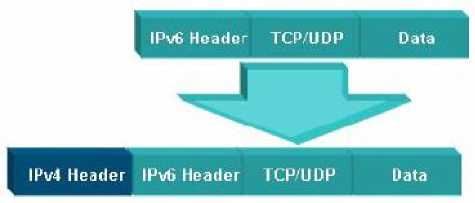
Fig.1. Tunneled IPv6 Packet

The use of tunneling comes with several shortcomings like high header overhead as a result of adding several protocol headers in a packet which results in low efficiency and performance degradation, especially over wireless links where resources are scarce [5]. Using header compression techniques we can improve the efficiency of tunneling mechanism. Header compression deals with compressing the excess protocol headers over the link and decompressing it at the other end of the link [6]. Most of the information in the header is static, like source address, destination address etc, or varies in a specific pattern, like identification field, TTL etc. These packet headers are very important over end to end communication but of very importance from one hop to another. So, it’s better to use header compression, which would result in many cases more than 90% savings, and thus save the bandwidth and use the expensive resources efficiently [7]. Using header compression we are increasing the computational complexity, but the compression gains are so high, so that we can compromise on the complexity. Bandwidth is the most costly resource in cellular links. Processing power is very cheap in comparison. Implementation or computational simplicity of a header compression scheme is therefore of less importance than its compression ratio and robustness [8]. Table 1 show the header compression gains which can be achieved using header compression over different protocol headers [9].

Table 1. Compression Gains

Protocol headers	Total header size (bytes)	Minimum Compressed header size (bytes)	Compression gain (%)
IPv4/TCP	40	4	90
IPv4/UDP	28	1	96.4
IPv4/UDP/RTP	40	1	97.5
IPv6/TCP	60	4	93.3
IPv6/UDP	48	3	93.75
IPv6/UDP/RTP	60	3	95

Rest of the paper is structured as follows: section II describes about the Literature survey, section III discusses about the proposed methodology, section 3 describes about the Simulation parameters and scenario. Results are discussed in section 4, section 5 concludes the paper.

• II.    Literature Survey

• [10]    Proposed a new technique called as Routing-Assisted Header Compression (RAHC) for end-to-end header compression technique for multi-hop wireless ad hoc networks. RAHC works in conjunction with conventional on-demand routing techniques and relies on the information provided by the routing algorithm. Here partial flooding is used for updating the context information for the nodes that lie between source & destination. The failure of intermediate node may result in de-synchronization of the source and destination nodes. In this case routing algorithm initiates route discovery and the context information has to be updated in all the nodes that have been newly introduced into the path. [11] Proposed a new approach for header compression in conjunction with IP security framework. Here the IPv6 protocol header is compressed and the benefit is a reduction of the overhead caused by IPSec tunnel mode in terms of enlarged datagram’s. [12] Proposed the approach of end to end header compression over wireless mesh networks. Here packet aggregation scheme is used in cooperation with the header compression mechanism. Simulations shows that only using a suitable header compression scheme can optimize the bandwidth usage in VoIP applications over wireless mesh networks, impacting positively in the loss packet. [13] Proposed the use of header compression in context of IP based ITS communication. Here our kernel implementation of an

open source RoHC library is described. This integration of a RoHC library inside the kernel may also be an advantage in terms of dynamic adaptation. [14] Proposed a new header compression mechanism which can be deployed in end-to-end nodes using the Software-Defined Network concept. Using this mechanism can reduce both packet size and time delay. In addition to utilize the use of the network, it also benefits in time factor for an application that requires low latency and small packet size such as VoIP. [15] Proposed the usage of traffic optimization techniques within the context of the LISP (Locator/Identifier Separation Protocol) framework. These techniques use Tunneling, Multiplexing and header Compression of Traffic Flows (TCMTF) in order to save bandwidth and to reduce the amount of packets per time unit. Using this approach bandwidth can be drastically reduced. [16] Proposed a new technique for header compression scheme ROHC+ for TCP/IP streams in a wireless context, such as the 3G platform, characterized by relatively high loss. Results show that the new header compression provides an efficient use of radio resource with direct benefit on the economic feasibility and on the quality of the service.

• III.    Proposed Methodology

In this paper we are compressing only the IPv6 header of the packet, as it is of largest length of 40 bytes. We have classified the header fields of IPv6 packet as STATIC, DYNAMIC, and INFERRED [17].

STATIC: Static fields are the header fields which remain unchanged during the life time of a header. These fields are sent only with uncompressed packets.

DYNAMIC: These are the fields which change in a specified pattern or randomly. These fields are compressed efficiently, i.e. Identification field in IPv4 header.

INFERRED: These fields are never sent within a packet and they are inferred from the lower layers in the protocol stack, like Total length in IPv4 packet.

The following table: 2 classify the header field in the IPv6 header:

Table 2. Header Classification for IPv6 Header

Protocol Field	Classification
Version	STATIC
Flow label
Next Header
Source IP Address
Destination IP Address
Traffic Class	DYNAMIC
HOP Limit
Payload Length	INFERRED

At Sender side:

At the network layer we have added a new parameter called tunnel algo to use. It takes the value 0 or 1. Based on this value we are deciding which mechanism to use, either compresses or uncompressed. It tunnel algo to use is 0: specifies normal tunneling mechanism is used. If it is set to 1: specifies compressed tunneling mechanism to use. Along with this, we are taking a value n, where n is number of uncompressed packets to send. Here initially we are sending first n packets uncompressed in the tunnel, and adding two extra bytes, in these uncompressed packets. This extra byte represents the C_ID and P_ID of the packet and is known as context header. The structure of this context header is shown in figure: 2.

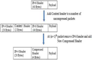
Fig.6. Handling packet at sender side

P_ID (8 bits)

C_ID (8 bits)

Fig.2. Context Header

Where, Profile ID (P_ID) represents the different profiles and these profiles need to be decompressed according to the profile id specified. Currently the profile specified is IPv6 only profile.

Context ID (C_ID) represents the context on the basis of which we can identify different flows in router.

Adding this context header we are adding two extra bytes and increasing the header overhead, but this context header is added only to n uncompressed packet, we call it context packets which are needed to establish context between the edge routers. The format for context header packet is shown in figure: 3. We are sending n context packets to the destination edge router.

IPv4 Header 0C Bytes)

Context Header (2 bytes)

IPv6 Header (40 bytes)

Pay load

Fig.3. Context Packet

At Destination side:

At the dual stack router (edge router) receives the IPv6 packet whose destination address is its own address it does the following:

IPv4 header is striped off from the packet.

For n uncompressed packets

First remove the context header after reading the values of p_id and c_id.

Read static info from the IPv6 packet and stores the information for corresponding c_id and send the packet to the intended destination.

At n+1 packet

Read compressed header to get p_id and c_id.

Check the static entry for this corresponding c_id.

Make a new IPv6 header based on this static and dynamic information.

Add this new IPv6 header in front of the packet.

This IPv6 packet is routed onto the IPv6 LAN toward the destination address as specified in the IPv6 packet.

The following figure 7 and figure 8 specifies the handling of packet at the destination:

Once n packets are sent, then we remove the IPv6 header from the packets and add the new compressed header before encapsulating inside the IPv4 packet. The format of compressed header is shown in figure: 4.

Pi о file ID (8 bits)

Ё С out ext ID (8 bits)

HopLimit (8 bits)Traffic Class (8 bits)P Ten (16 bits)

Fig.4. Compressed Header

Here Profile_ID and Context_ID are derived from the context header and remaining fields are the dynamic and inferred fields which are sent with every compressed packet. The format for compressed packet is shown in figure: 5.

IPv4 Header (20 Bytes )

Compressed Header (6 bytes)

Payload

Fig.5. Compressed Packet

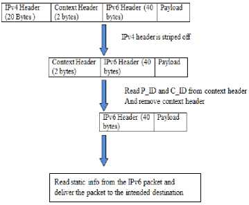
Fig.7. Handling n packets

We are sending compressed packet until the simulation ends. Figure 6 specifies the working at the sender side:

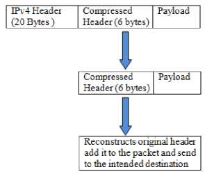
Fig.8. Handling n+1 packets

Performance of most of the header compression algorithm degrades because of context updation. These algorithms use different context updation mechanisms like interval context updation, or updation in case of packet losses. The advantage of our algorithm is that there is no need of context updation, since all the dynamic and inferred information is carried in packet headers, which would result in lower compression gain, but the benefit of this, is that there is no need of context updation. If a packet is lost, it does affect the successful decompression of subsequent packets.

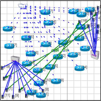
Fig.9. Scenario for Simulation

The following table-3 shows the simulation parameters for this scenario.

• IV.    Simulation Test Bed

Simulations play a vital role in testing our network scenarios and specify the network parameters. A scenario allows the user to specify all the network components and conditions under which the network will operate. These conditions can be terrain details, channel properties, networking devices, and the properties of entire protocol stack. Different Simulators are available like NS-2, NS-3, Opnet, GNS 3, Exata/Cyber, Qualnet etc. We have used Qualnet 5.1 to simulate our protocol. QualNet 5.1 provides a comprehensive environment for designing protocols, creating and animating network scenarios, and analyzing their performance [18]. Figure 9 represents the scenario of our network. Here network is a hybrid network which consist of both wired and wireless subnets, where backbone routers are wireless routers and the end users are wired network. Here a tunnel is created between the edge routers of both the networks, router 3 and 5 are dual edge routers for two IPv6 networks. Here tunnel is a Multihop wired tunnel, and all the intermediate routers are IPv4 only routers i.e. they understand IPv4 only packets and discard IPv6 packets. Since it is a end-to-end algorithm, it means compression and decompression is performed only at the edge routers i.e. at router 3 and router 5, and other routers forward the packets without performing compression and decompression. Here simulations are carried out by varying the bandwidth of wireless network from 500 kbps to 5 mbps. After 5 mbps network conditions are stable for compressed and uncompressed network. So the further results are not taken into consideration.

Table 3. Simulation Parameters

Parameter	Value
Simulator	Qualnet 5.1
Studied Protocol	Bellman Ford for IPv4 Networks.
	RIPng for IPv6 Networks.
Area	1500m x 1500m.
Total no. of nodes	42 nodes.
Dual Stack Edge Nodes	02
IPv4 only nodes	22
IPv6 only nodes	18
No. of Packet Sources.	04
Bandwidth for wireless network	500 KBPS, 1 MBPS, 2 MBPS, 3 MBPS, 4 MBPS, 5 MBPS.
Bandwidth for wired network	10 MBPS
Type of sources	Constant Bit Rate (CBR)
MAC protocol	802.11 for Wireless Networks 802.3 for Wired Networks
Packet size	512 Bytes
Traffic Rate	100 packet per second
Mobility model	None
Simulation time	300 seconds
Channel type	Wired & Wireless.
Antenna model	Omni Directional
No. of Simulations runs	12 runs

• 5.1.    Throughput

Results are simulated on Qualnet 5.1 Simulator, here comparisons is done on the basis of varying bandwidth of wireless network. Header compression is done over Multihop wireless tunnel and 4 Constant Bit rate (CBR) applications are used on varying bandwidth of 500 KBPS, 1 MBPS, 2 MBPS, 3 MBPS, 4 MBPS, and 5 MBPS. We have done comparisons for compressed and uncompressed network. The metric based analysis is shown in table 4 to 7 and figure 10 to 13.

Throughput can be defined as the number of packets delivered per unit time. More the bandwidth greater the throughput will be for any network. It is measured in bits/sec. Here we are analyzing throughput for varying bandwidth of wireless network. The formula for throughput is given as:

Throughput (T) = 8*Total No. of Bytes Received/ (time last packet sent - time first packet sent)

Figure 10 depicts the graph for throughput. We are getting highest throughput when the bandwidth is 5 mbps, since more the bandwidth greater the throughput will be. Throughput is very less in case when bandwidth is 500 kbps. From the graph it is clear that every time we are getting better results is case of compressed network. Here we can say that bandwidth is proportional to throughput, i.e. as bandwidth increases, throughput increases considerably.

Bandwidth (B) ∝ Throughput

Table 4. Throughput

Throughput (bits/s) Bandwidth Uncompressed Compressed 500 KBPS 9362 13169 1 MBPS 30451 33847 2 MBPS 122506 164379 3 MBPS 281281 298649 4 MBPS 389871 409606 5 MBPS 407710 409603 calculation is given as:

Average end-to-end delay = (total of transmission delays of all received packets) / (number of packets received), where, transmission delay of a packet = (time packet received at server - time packet transmitted at client) , where the times are in seconds.

Figure: 11 depicts the graph for Average End-to-End Delay. Result shows that average end-to-end delay is very high for low bandwidth i.e. 500 kbps, but as the bandwidth increases average end-to-end delay decreases considerable and is almost negligible when bandwidth is 5 mbps. But still we are experiencing less delay in case of compressed networks. Here we can say that average end-to-end delay is inversely proportional to bandwidth, i.e. as bandwidth increases, average end-to-end delay decreases considerably.

Bandwidth (B) ∝ 1/ End-to-end delay

Table 5. Average-end-to-end delay

Average End-to-End Delay (s)
Bandwidth	Uncompressed	Compressed
500 KBPS	30.0944	25.4849
1 MBPS	12.6209	12.1964
2 MBPS	3.48059	3.45001
3 MBPS	1.85479	1.86619
4 MBPS	0.865408	0.0178829
5 MBPS	0.0154019	0.014862

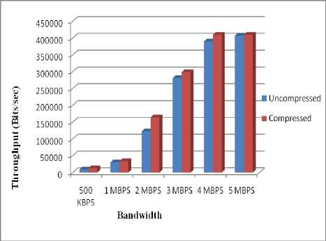
Fig.10. Throughput Vs Bandwidth

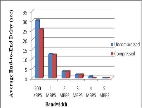
Fig.11. Average End-to-End Delay Vs Bandwidth

• 5.2.    Average End-to-End Delay

• 5.3.    Average Jitter

Average end-to-end delay is the time interval between the packets is sent by the source node and is received by the destination node. All different delays are included like propagation delay, queuing delays, delay for route discovery, etc. Delay is an important factor for finding the network performance. Delay should be less as the packets must reach from source to destination in very less time. It is calculated in seconds. The formula for delay

Jitter is defined as the variation in the arrival time between two consecutive packets. Jitter is measured in secs, and it should be very less. For real time applications jitter should be negligible, for better experience. The formula for Jitter calculation is given as:

Average jitter = (total packet jitter for all received packets) / (number of packets received - 1)

where, packet jitter = (transmission delay of the current packet

• - transmission delay of the previous packet).

Jitter can be calculated only if at least two packets have been received.

Figure:  12 depicts the graph for average jitter.

Simulations show that jitter is almost negligible when bandwidth is 5 mbps. But as the bandwidth decreases its impact is shown over the jitter, it increases significantly. We are experiencing less delay in case of compressed network, as we are reducing the overall size of the packet. Jitter is improved in case of our algorithm. Here we can say that bandwidth is inversely proportional to average jitter, i.e. as bandwidth increases, average jitter decreases considerably.

Bandwidth (B) ∝ 1/ Jitter

Table 6. Average Jitter

Average Jitter (s)
Bandwidth	Uncompressed	Compressed
500 KBPS	0.629625	0.5484
1 MBPS	0.206304	0.19234
2 MBPS	0.0332409	0.0294222
3 MBPS	0.011667	0.0105134
4 MBPS	0.00487796	0.000681807
5 MBPS	0.000647171	0.000631304

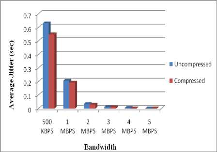
Fig.12. Average Jitter Vs Bandwidth

• 5.4.    Packet Delivery Ratio (PDR)

It is the ratio of number of packets actually delivered from source to destination, to the number of packets sent. PDR should be high for better performance, Higher the PDR, more the throughput. The formula for packet delivery ration is given as:

PDR = (Total number of Packets Received / Total number of Packets Send) *100.

Figure: 13 depict the graph of Packet Delivery Ratio. From the graph it is clear that PDR is almost 100% when bandwidth is 5 mbps, but as the bandwidth decreases, PDR declines. Because when the bandwidth is high link utilization is effective, as the bandwidth decreases, packet are dropped which degrades the PDR, and its affect is shown over other parameters. Here we are getting better results in compressed networks. Here we can say that bandwidth is proportional to PDR, i.e. as bandwidth increases, PDR increases considerably.

Bandwidth (B) ∝ Packet Delivery Ratio

Table 7. Packet Delivery Ratio

Packet Delivery Ratio
Bandwidth	Uncompressed	Compressed
500 KBPS	2.284444444	3.213333333
1 MBPS	7.433333333	8.262222222
2 MBPS	29.90666667	40.12888889
3 MBPS	68.66888889	72.90888889
4 MBPS	95.18	99.99777778
5 MBPS	99.53555556	99.99777778

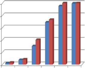
■ Uncompressed

■ Compressed

500 1 MBPS 2MBPS 3 MBPS 4 MBPS 5MBPS

KBPS

Bandwidth

Fig.13. Packet Delivery Ratio Vs Bandwidth

• VI. Conclusion

IPv6 is the future of the internet without which it’s not possible to sustain internets life. In this paper we have proposed a new approach for improving the efficiency of IPv6 tunneling mechanism which results in the betterment for enabling the smooth interoperation of the two protocols. Using this approach we have compressed the 40 bytes of IPv6 header up to 6 bytes, which is significantly a big improvement. Compressing the IPv6 header we are getting better network deliverables in terms of throughput, average end-to-end delay, Jitter, and Packet delivery ratio. We have compared the result with normal tunneling mechanism. Simulation is carried out over Qualnet 5.1 simulator. Results shows that a compressed network performs better results than uncompressed network. Currently we are simulating it over small networks with limited load, even better results could be achieved if applied to large scale networks. Bandwidth is the most critical resource for a network and it must be utilized efficiently. Here we are better utilizing the bandwidth using header compression. Currently we are having only one profile i.e. IPv6 only profile, later on IPv6/UDP and IPv6/TCP would be added to our work.