Advances in Malware Detection using Machine Learning and Deep Learning: A Comprehensive Comparative Analysis

Rapid proliferation and increasing sophistication of malware present a persistent and escalating threat to digital security worldwide. Traditional signature-based detection methods, which rely on matching known patterns, are increasingly ineffective against polymorphic malware, zero-day exploits, and advanced obfuscation techniques. This requires the development of more robust and adaptable solutions capable of detecting and classifying previously unseen threats. Machine learning and deep learning have emerged as powerful tools for malware analysis, offering the potential to automatically learn complex patterns and discriminate between benign and malicious software with greater accuracy and efficiency. offer comprehensive overviews of the evolution and current state of ML-powered malware detection. This research article conducts a detailed comparative analysis of machine learning and deep learning models for malware classification, focusing on both theoretical foundations and practical implementations. We evaluated a diverse set of Machine Learning algorithms, such as Random Forest, Logistic Regression, AdaBoost, and Deep Learning architectures, including Recurrent Neural Network, Long Short-Term Memory, Gated Recurrent Unit, bidirectional LSTM, and eXtreme Gradient Boosting. These models are trained and tested on diverse datasets and incorporate features derived from static, dynamic, and hybrid analysis approaches. As highlighted in [1], feature engineering and selection play a crucial role in the performance of machine learning-based malware detection, while [2] explores the particular strengths and challenges associated with applying different Deep Learning models in this domain. introduces the motivation to use deep learning techniques in malware analysis due to the increase in malware instances. This study goes beyond simply comparing the accuracy of the model. We investigate the impact of feature selection methods, both traditional techniques such as L1 regularization and more advanced strategies such as Genetic Algorithms [3, 4], on the performance of Machine Learning and deep learning models. We assess the resilience of models to adversarial attacks, recognizing the growing threat of attackers trying to evade machine learning-based defenses [5, 6]. Furthermore, we address the practical considerations of deploying these models in real-world settings, including computational resource constraints and the need for explainable AI to foster trust and understandability [7].

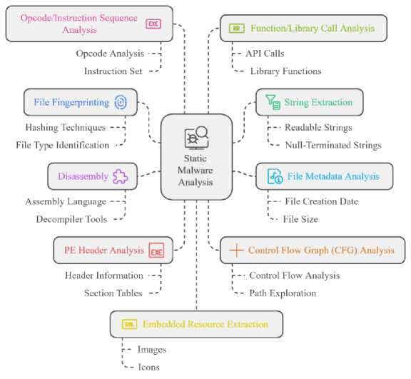
Fig.1. Taxonomy of static malware analysis

This research evaluates machine learning and deep learning models for malware classification using EMBER and Microsoft Big 2015 datasets. It analyzes how feature selection impacts model performance and explores deep learning’s capacity for automated feature learning. The study also assesses model robustness against adversarial attacks designed to preserve malicious functionality, offering practical recommendations for deploying these models in real-world malware detection systems. Key considerations include accuracy, computational cost, and explainability. The goal is to provide insights for researchers and practitioners, emphasizing the importance of publicly available datasets, benchmark comparisons, and advanced deep learning techniques for enhancing malware detection systems.

2.    Taxonomy of Malware Analysis

Malware analysis involves studying the functionality, origin, and impact of malicious software. Four key approaches are employed: static analysis, which examines code without execution to identify indicators; dynamic analysis, which involves executing malware in a controlled environment to observe real-time behavior; behavioral analysis, an extension of dynamic analysis that focuses on the overall system impact by monitoring network traffic and system changes; and hybrid analysis, which combines both static and dynamic methods for a comprehensive understanding. Collectively, these approaches form a robust framework for identifying, understanding, and mitigating malware, thereby enhancing cybersecurity defenses.

• 2.1.    Static Analysis

• 2.2.    Dynamic Analysis

• 2.3.    Hybrid Analysis

3.    Related Works

This approach examines the structural and syntactic properties of a malware sample without executing it. This includes examining headers, file signatures, API calls, strings, and other metadata to identify malicious characteristics [8, 9]. This approach offers advantages in terms of safety, as the malware is not executed, reducing the risk of system infection. Through static analysis, researchers can study the malware’s code, structure, and characteristics without causing harm, providing a thorough understanding of its functionality, behaviors, techniques, and potential impact. Key aspects of this methodology include file fingerprinting, string extraction [9], file metadata analysis [10] , disassembly [11], PE header analysis [9], control flow graph analysis [12], opcode/instruction sequence analysis [13], function/library call analysis [14], embedded resource extraction, signature-based detection, entropy analysis [15], embedded code extraction [16], cross-referencing with known malware databases, pattern matching and hexadecimal / binary code inspection [17].

Dynamic analysis involves executing the malware sample in a controlled, isolated environment and observing its runtime behavior. This allows for monitoring the malware’s actions, such as file modifications, network communications, API calls, and other behaviors that may not be evident from static analysis alone. Key aspects of this methodology include process monitoring, network traffic capture, file system monitoring, API call monitoring, memory analysis, registry monitoring, and sandbox analysis. By observing malware in a controlled setting, researchers and security professionals can gain insights that are impossible to obtain through static analysis alone. Dynamic analysis encompasses techniques like sandbox execution, behavioral monitoring [18], API call tracing [19], network traffic analysis [20], file system monitoring, process creation monitoring [12], registry monitoring, memory analysis [21], system call monitoring, dynamic instrumentation, virtual machine analysis, debugging, heuristic analysis, system change capture and analysis, and automated behavioral analysis tools [18].

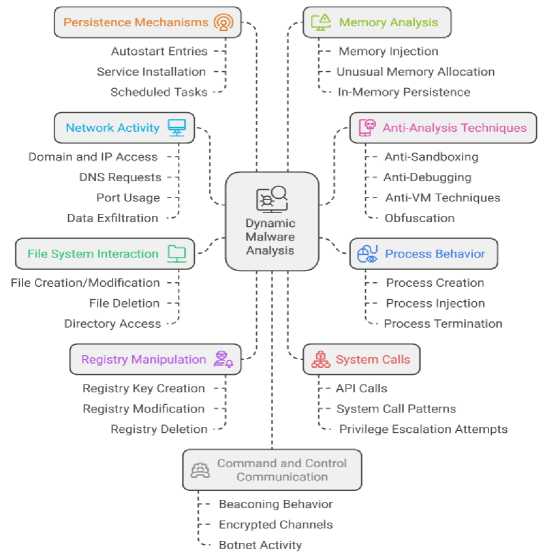
Fig.2. Taxonomy of dynamic malware analysis

However, dynamic analysis is limited by anti-analysis techniques [22], where malware detects the sandbox environment and changes its behavior or stops functioning altogether, making it more challenging to analyze. The combination of static and dynamic analysis, known as hybrid analysis, can lead to a more comprehensive understanding of malicious programs and enable researchers to gather a broader set of features for classification [23]. This approach takes advantage of both techniques, allowing for a more thorough examination of the behavior and characteristics of malware [24]. Static analysis can provide insights into the malware’s structure, code, and potential functionality, while dynamic analysis can reveal its runtime behavior, interactions, and impact on the system. By integrating these complementary methodologies, security researchers can gain a deeper understanding of malware, enabling the development of more effective detection and mitigation strategies.

Metamorphic and polymorphic malware present significant challenges to traditional signature-based detection due to their ability to dynamically alter their code structure and appearance while retaining malicious functionality [25]. Metamorphic malware rewrites its entire code with obfuscation techniques like code reordering and instruction substitution. Polymorphic malware modifies surface-level characteristics such as file names, checksums, and byte patterns, often through encryption with a decryption engine, making each instance appear unique. These evasive tactics necessitate advanced analysis methods, including machine learning and deep learning. Analyzing such malware is challenging but combining advanced dynamic and static analysis techniques is crucial [26]. Hybrid analysis, which starts with static feature extraction and then dynamic execution in controlled environments, offers a comprehensive understanding of malware behavior, addressing the limitations of individual methods [27]. While computationally intensive and potentially hindered by sophisticated packing [28], integrating static analysis for unpacking routines and dynamic analysis for unpacked code, alongside machine learning advancements, leads to robust detection and classification frameworks for evolving cyber threats.

The use of machine learning techniques has become increasingly prevalent in malware analysis, offering robust and scalable solutions for malware identification and classification; this provides a comprehensive review of research developments and trends in the area, categorizing methods based on the target task, feature types, and machine learning algorithms employed. Furthermore, it explores challenges and considerations in applying machine learning for malware detection, such as the need for representative datasets, performance maintenance over time, and model interoperability. Researchers have explored a wide range of machine learning algorithms for malware classification, including logistic regression, support vector machines, decision trees, random forests, naive Bayes, K-nearest neighbors, and gradient boosting classifiers. These traditional machine learning models have demonstrated promising results in accurately identifying malicious and benign files, often relying on a combination of static and dynamic features extracted from PE files.

Table 1. Comprehensive comparative study on Malware detection: methods, models, dataset and results

No.	Study	Methods Used	ML/DL Algorithm	Dataset	Results
1	Laouadi et al. [10]	Image conversion, MinHash, LSH, similarity-based classification	Two-phase malware detection	Undisclosed	97.53% training accuracy, 90.08% validation accuracy
2	Ganesh Sundarkumar et al. [29]	API calls, topic models, imbalance handling	Multi-Layer Perceptron, SVM, Decision Trees, Random Forest	Two datasets (imbalanced and diverse)	High sensitivity up to 98.61%
3	Li and Zheng [30]	API call sequences, Recurrent Neural Networks	LSTM, GRU	Malware families dataset	41%–55% accuracy, F1-scores 0.70 for Adware and Viruses
4	Akhtar et al. [31]	Comparative study with log data	Decision Tree, CNN, SVM	CIC dataset	99.01% accuracy, 0.021% false positive rate
5	Zhang et al. [32]	Deep learning on packed malware	Deep Belief Network (DBN)	Packed/unpacked malware dataset	High classification accuracy
6	Schultz et al. [33]	Data mining, supervised learning	Naive Bayes, Multi-Naive Bayes	Dataset of 3,301 executables	97.76%–98.59% accuracy
7	Santos et al. [34]	Opcode sequence analysis	Decision Trees, SVM	1,200 malwares, 1,200 benign samples	Decision Tree 96.65%, SVM 98.14% accuracy
8	Raff et al. [21]	Sequential pattern detection	Long Short-Term Memory Networks (LSTM)	Dataset of 1 million PE files	94.2% accuracy
9	Hou et al. [35]	System call graphs, Graph Convolutional Networks (GCN)	GCN-based malware detection	Android malware dataset of 87,000 samples	97.8% accuracy
10	Anderson and Roth [36]	Static feature analysis	Gradient Boosting Machines	Ember dataset	98.2% accuracy
11	Huang, Xu, and Zhang [32]	DNN ensemble with domain knowledge	Ensemble of Deep Neural Networks	80,000 samples	97.7% accuracy, adversarial vulnerabilities noted
12	Yerima and Sezer [37]	Android malware detection	Random Forest	100,000 Android applications	99.1% accuracy
13	Hardy et al. (DL4MD) [38]	Feature extraction via CNNs	Convolutional Neural Network	200,000 malware samples	98.6% accuracy
14	Demetrio et al. [39]	Adversarial learning	Adversarial attack techniques on deep learning models	Dataset of 150,000 PE files	Model performance varies with robustness against adversarial attacks
15	Shaukat, Luo, Varadharajan [40]	Image-based feature extraction, RegNetY320 model	RegNetY320, PCA for feature selection	Malimg dataset	99.30% accuracy
16	Gulsade Kale et al. [41]¨	Genetic algorithms for feature selection	Multi-objective Genetic Algorithms (MOGAs)	Comparative dataset	93.33% classification accuracy, 40% performance improvement
17	Rudd et al. [42]	Metric learning with triplet loss	Neural network with metric learning	Malware benchmark datasets	State-of-the-art accuracy, computationally intensive

Shaukat, Luo, and Varadharajan [40] propose a framework that transforms Portable Executable files into images and uses a pre-trained deep learning model for feature extraction, achieving 92% accuracy and a 92.16% F1 score. Laouadi et al.[10] present a two-phased approach using image conversion and machine learning, with the static analysis phase reaching 97.53% training accuracy and 90.24% validation accuracy, excelling at identifying novel malware. Vinayakumar et al. [43] evaluated several machine learning algorithms on the EMBER dataset, finding that Random Forest achieved the highest accuracy of 88.66%, with a precision of 81.74%, recall of 97.81%, and F1-score of 89.06%. These findings highlight the potential of both deep learning and ensemble methods in capturing complex patterns in malware samples.

Ganesh Sundarkumar et al.[29] explored a machine learning approach to malware detection, evaluating their methodology on both imbalanced and diverse datasets. Their work showcased high sensitivity rates across several classifiers, with Multi-Layer Perceptron achieving an impressive 98.61% sensitivity. The study emphasized the importance of sensitivity and specificity, with the Decision Tree classifier emerging as a preferred model due to its high sensitivity and interpretable rules. The consistent results across different datasets underscored the robustness of their proposed methodology. Li and Zheng [30] investigated malware classification using API call sequences and Recurrent Neural Networks, specifically LSTM and GRU models. While their experiments demonstrated promising accuracy levels (41% to 55% for LSTM and 48% to 55% for GRU), the study also highlighted the challenge of inconsistent performance across different malware families. The models performed well in detecting Adware and Viruses but struggled with Trojans and Spyware, indicating the need for further refinement and a more comprehensive evaluation of their approach’s effectiveness. Akhtar et al.[31] delved into the application of machine learning for malware identification and analysis, comparing Decision Tree, CNN, and Support Vector Machines. Their results highlighted the superiority of the Decision Tree model, which achieved a remarkable 99.01% accuracy and a low false positive rate of 0.021. This research underscores the potential of machine learning, particularly Decision Tree algorithms, as a robust and effective approach for combating the growing threat of malware.

Zhang et al.[32] propose using Deep Belief Networks, a deep learning approach, to effectively detect packed malware variants that can evade traditional methods. DBNs can automatically learn complex patterns from raw binary data, addressing the limitations of manual feature engineering in prior studies. Their approach, trained on packed and unpacked malware, demonstrates high accuracy in classifying new, unseen malware variants. While the results are promising, the authors acknowledge the need to evaluate the method on larger, more diverse datasets and enhance its robustness against adversarial attacks. Nevertheless, the work highlights the potential of DBNs as a powerful tool for combating the growing prevalence of packed malware. Schultz et al.[33] investigates the use of data mining techniques for detecting new malicious executables. Analysing a dataset of 3,301 executable, the researchers applied Naive Bayes and Multi-Naive Bayes classifiers, achieving impressive accuracies of 97.76% and 98.59%, respectively. However, the study’s limitations include the relatively small dataset size and the use of simple machine learning models, which may not adequately capture the complexities of more advanced malware techniques. In contrast, the work by Anderson et al. explores the use of more sophisticated machine learning models, such as Support Vector Machines and Random Forests, for malware classification. Santos et al.[34] investigated the use of Decision Trees and Support Vector Machines to detect malware by analyzing opcode sequences from executable files. Utilizing a dataset of 1,200 malware and 1,200 benign samples, the Decision Tree model achieved 96.65% accuracy, while the SVM model reached 98.14% accuracy. However, the authors note that the sole reliance on opcode sequences presents a limitation, as advanced malware can employ obfuscation techniques to evade detection based on these sequences. This research highlights both the potential and the challenges of opcode-based malware detection methods in cybersecurity.

Rieck et al. [44] approach combines clustering and classification, with a particular focus on SVM for classification tasks. The study is based on a substantial dataset of 100,000 malware samples from public repositories, providing a robust foundation for model training and evaluation, the study also highlights a notable limitation: the high computational cost associated with dynamic analysis. This process of executing malware in a controlled environment to observe its behaviour can be resource-intensive and time-consuming. Kolosnjaji et al. [45] utilize Deep Neural Networks (DNNs) to analyze sequences of system calls, leveraging their ability to capture complex patterns within sequential data. The study is based on a dataset comprising 40,000 samples, evenly divided between 20,000 malware samples and 20,000 benign samples. The DNN-based approach achieves a notable accuracy of 95.85, demonstrating the high efficacy of deep learning in distinguishing between malicious and benign activities. However, the research also identifies a significant limitation: the limited interpret ability of deep learning models. While DNNs provide high classification accuracy, their “black box” nature makes it challenging to understand and explain their decision-making process. This issue of interpret ability is a critical consideration for enhancing the trustworthiness and usability of deep learning models in cyber security applications. Saxe and Berlin [46] present an approach involves analyzing two-dimensional binary features extracted from executable, allowing the deep learning models to capture complex patterns and relationships within the binary code. The study is based on an extensive dataset of 400,000 executable files, providing a solid foundation for model training and evaluation. The deep neural network approach demonstrates a high accuracy rate of 95.5, highlighting its effectiveness in distinguishing between benign and malicious software. However, the research also identifies a significant limitation: the potential for over fitting due to the large number of parameters in the deep neural network models. This risk of overfitting could lead the model to memorize the training data rather than generalize to new, unseen data, potentially affecting the robustness of the detection system. Despite this challenge, the paper underscores the substantial potential of deep learning techniques in malware detection and emphasizes the need for strategies to address over fitting, enhancing model generalization.

Raff et al.[47] propose an LSTM-based approach for malware detection, achieving 94.2% accuracy by analyzing sequential patterns in executable files. Though their method utilizes a large dataset of 1 million PE files, the research highlights the significant computational resources required for training the LSTM models. Despite this challenge, the paper demonstrates the potential of LSTM networks in enhancing malware detection and emphasizes the need to address computational constraints to improve the practicality of such advanced techniques. Hou et al. [35] presents a deep learning-based malware detection framework using Graph Convolution Networks that analyzes system call graphs from Android apps to identify malicious behavior. Their approach achieves 97.8% accuracy on a dataset of 87,000 samples. However, the framework is limited to Android and may not address malware detection challenges on other platforms. The research highlights the need for further work to extend the GCN-based approach to a more versatile, cross-platform solution. Anderson and Roth [36] present a valuable resource for malware detection research through the Ember dataset and demonstrate high-performing gradient boosting techniques for classifying Portable Executable files based on static features. Their approach achieves 98.2% accuracy, but is limited to static analysis, potentially missing certain malware types. Huang, Xu, and Zhang [48] present a sophisticated malware detection approach using an ensemble of Deep Neural Networks integrated with domain-specific knowledge. Their ensemble method achieves a notable accuracy of 97.7% in distinguishing between benign and malicious software. However, the study identifies the system’s susceptibility to adversarial attacks as a key limitation, highlighting the need to address this vulnerability to improve the security and robustness of malware detection methodologies.

Yerima and Sezer [37] present a machine learning-based method for detecting Android malware, leveraging the Random Forest algorithm to analyze application permissions and API calls. Their approach achieves a high accuracy of 99.1% in identifying malicious Android apps, but is limited to the Android platform, emphasizing the need for similar studies across multiple operating systems. Hardy et al. [38] present an advanced framework utilizing Convolutional Neural Networks to enhance malware detection. Their DL4MD framework achieves an impressive accuracy rate of 98.6%, demonstrating the significant potential of CNNs in improving malware detection and analysis. However, the research acknowledges the black-box nature of deep learning models, which impedes interoperability and underscores the need for further research into enhancing model transparency. Demetrio et al.[39] investigates the susceptibility of deep learning models to adversarial attacks in malware detection. Their study highlights the high computational cost associated with generating adversarial examples and sheds light on the vulnerabilities of deep learning models, underscoring the need for developing more robust and efficient malware detection methods. David and Netanyahu [49] present a deep learning based approach called DeepSign, which utilizes auto-encoders to automatically generate malware signatures and classify malware samples. DeepSign achieves a high accuracy of 96.3% on a large dataset of 500,000 malware samples, but the research also highlights a limitation of the model’s ability to handle novel or significantly different malware variants, which could impact its performance in dynamic threat landscapes.

Sethi et al.[50] presents a hybrid framework that extracts features from both executable files and runtime behavior, achieving high accuracy but acknowledging limitations in dataset size and potential bias. They suggest evaluating the framework on larger, more diverse datasets and exploring deep learning techniques for enhanced feature extraction and classification. Balram et al. [9] investigates static malware analysis on the APT1 dataset, comparing multiple classifiers and feature categories like strings and PE header information. They achieve high accuracy with low processing time but recognize dataset specificity and bias as limitations. Future work should evaluate the approach on more diverse datasets and explore additional features for improved generalization and robustness. Ismail et al.[51] propose a machine learning based approach to enhance real-time network-level malware detection, combining signature-based detection and machine learning. Their method achieves comparable accuracy to stateful methods while minimizing resource consumption but is limited by dependence on known signatures and potential evasion by obfuscated malware.

Gulsade Kale et al. [41] present a novel approach to enhance malware detection using multi-objective genetic algorithms for feature selection. The study recognizes the limitations of traditional signature-based methods and emphasizes the importance of refined feature sets to improve detection performance. The researchers evaluate various machine learning classifiers and find that MOGAs effectively optimize the feature selection process, leading to a 93.33% classification accuracy and a 40% performance improvement. The detailed evaluation using statistical analysis further validates the findings, highlighting the potential of advanced feature engineering techniques in strengthening machine learning-based malware detection systems. Kumar et al. [52] investigates malware classification using the CIC-MalMem-2022 dataset. The study employs six machine learning models: Logistic Regression, SVM, KNN, Random Forest, Naive Bayes, and Decision Tree, coupled with a correlation-based feature selection approach. The Decision Tree model achieved superior performance metrics, including accuracy (0.9994), precision (0.9996), recall (0.9992), and F1-score (0.9995) in training, and comparable results with KNN during testing. The research highlights the effectiveness of feature selection and the robustness of Decision Tree and KNN models in malware detection. Limitations include dataset imbalance and model generalization. Rudd et al.’s [42] work builds on advancements in machine learning for malware analysis. Traditional methods struggle with evolving threats, while machine learning offers a robust alternative, though reliance on handcrafted features limits scalability. Deep learning shows promise but requires substantial resources. Metric learning, the foundation of Rudd et al.’s work, learns a distance function to reflect semantic similarity, like in image retrieval, making it suitable for malware analysis. Rudd et al. use metric learning with a triplet loss function to train a neural network on raw binary data, achieving state-of-the-art accuracy, though the approach is computationally intensive. Future work should address interoperability of learned embeddings and generalization to unseen malware.

4.    Our Approach

This study performs a comparative analysis of machine learning and deep learning models for malware classification using the EMBER and Microsoft Big 2015 dataset. We evaluated a range of machine learning methods, including Logistic Regression, AdaBoost, Naive Bayes, and Decision Tree, alongside deep learning architectures, including recurrent neural network, long-short-term memory, gated recurrent unit, bidirectional LSTM, and eXtreme Gradient Boosting. These models are assessed both with and without feature selection methods to understand their impact on performance and efficiency. Performance is evaluated using accuracy, precision, recall, and F1 -score. The choice of these specific algorithms and architectures allows for a comparison of established baseline methods with more complex models designed to capture intricate patterns and temporal dependencies in malware data. This research aims to provide practical recommendations for malware detection system development by examining the trade-offs between model complexity, performance, and the benefits of feature selection. Recognizing the challenges posed by evolving malware tactics and the potential for adversarial attacks, the chosen models’ robustness and adaptability will also be considered. Our approach is visually summarized in Fig.3. This figure illustrates the workflow of our analysis, highlighting the different models, feature selection process, and evaluation metrics used in this study.

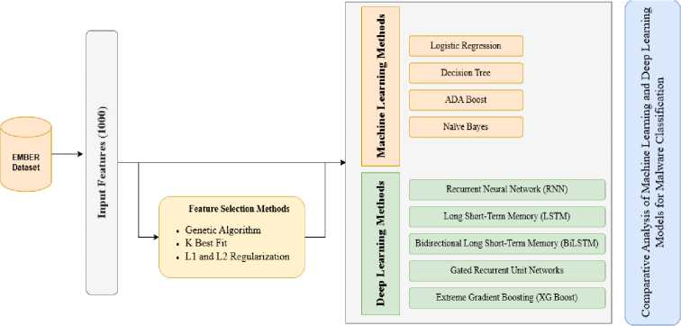
Fig.3. Machine learning and deep learning-based approach for classification and comparative analysis

• 4.1.    Feature Selection

Feature selection is crucial for effective malware classification, impacting accuracy, computational cost, and model interpretability. In this work three feature selection methods, namely, logistic regression with regularization, genetic algorithm, and select K-best, have been employed and analyzed with respect to their strengths and weaknesses.

• L1 and L2 regularization are employed with Logistic Regression for feature selection in malware detection. L1 regularization effectively removes less important features by driving their coefficients to zero, resulting in a sparser, more interpretable model that highlights the most influential features. L2 regularization shrinks coefficients towards zero without eliminating them, which helps to mitigate multicollinearity often present in malware datasets, thus improving model robustness and preventing overfitting [53].

• 4.2.    Dataset

  The Ember [36] and Microsoft Big 2015 [56] Dataset is a comprehensive resource for training machine learning models to classify Windows executable files as benign or malicious, featuring header, disassembly, string, entropy, byte sequence, API call, dynamic analysis, and statistical features, as well as malicious behavior indicators. The Microsoft BIG 2015 [56] dataset was also used for comparative analysis, offering raw byte/ASM features for evaluating model generalization and robustness across different feature engineering methodologies.

• 4.3.    Experimental Setup

5.    Results and Discussions

• 5.1.    Experimental Results on Malware Classification using Various Machine Learning Models

The Genetic Algorithms frame feature selection as an optimization problem where feature subsets, represented as “chromosomes,” evolve through processes like selection, crossover, and mutation. These processes are guided by a fitness function, typically based on classification performance metrics. This method is particularly effective for high-dimensional malware feature sets as it explores a vast search space to identify optimal or near-optimal feature combinations [54].

The Select K Best method ranks features based on statistical tests (e.g., chi-squared, ANOVA F-value) to measure their individual association with the target variable. The top K features are then chosen. While simple and computationally efficient for dimensionality reduction, this approach may overlook valuable feature interactions, and other methods might yield better results with specific machine learning algorithms [55].

The experimental setup utilizes the Ember dataset, which comprises a comprehensive collection of Portable Executable files. The analysis is performed using a train-test split of 300,000 samples for training and evaluation. The dataset includes both static and behavioral attributes. Static features include file metadata, byte patterns, and opcode sequences, while behavioral features may include API calls and system interactions. Various feature selection algorithms are used. This comprehensive setup allows for a comparative analysis of feature selection methods and their impact on predictive accuracy for malware detection within the Ember dataset.

The study leverages the Ember dataset, a comprehensive collection of Portable Executable files, to conduct a comparative analysis of feature selection methods and their impact on malware detection accuracy. The experimental setup involves a train-test split of 300,000 samples and encompasses both static and behavioral attributes. Feature selection algorithms such as Select K Best Fit and Genetic Algorithm are employed, along with regularization techniques like L1 and L2, to investigate their influence on predictive performance. This comprehensive approach enables researchers to gain valuable insights into the relative strengths and weaknesses of various feature selection methods in the context of malware detection using the Ember dataset.

This study compared the performance of four machine learning algorithms like Logistic Regression (Fig.4), Naive Bayes (Fig.12), Decision Tree (Fig.6), and AdaBoost (Fig.7) across different feature selection methods. The objective was to assess their validation accuracy and class-wise performance metrics, such as precision, recall, and F1-score.

As depicted in Fig.4, Logistic Regression exhibited stable and strong performance across all feature selection methods.

Table 2. Malware classification results using machine learning algorithms with different feature selection methods

Algorithm	Feature Selection Method	Model	Accuracy	Precision (Class 0)	Recall (Class 0)	F1-Score (Class 0)	Precision (Class 1)	Recall (Class 1)	F1-Score (Class 1)
Logistic Regression	L1 Regularization	-	0.90	0.87	0.90	0.89	0.92	0.90	0.91
	Genetic Algorithm	-	0.90	0.87	0.90	0.89	0.92	0.90	0.91
	K Best Fit	-	0.90	0.87	0.90	0.89	0.92	0.90	0.91
	All Features	-	0.90	0.88	0.91	0.89	0.93	0.90	0.91
Naive Bayes	L1 Regularization	Gaussian	0.63	0.72	0.27	0.39	0.61	0.92	0.73
		Bernoulli	0.66	0.68	0.42	0.52	0.64	0.84	0.73
	Genetic Algorithm	Gaussian	0.64	0.70	0.35	0.46	0.63	0.88	0.73
		Bernoulli	0.66	0.68	0.45	0.54	0.65	0.83	0.73
	K Best Fit	Gaussian	0.62	0.65	0.35	0.45	0.62	0.85	0.71
		Bernoulli	0.64	0.65	0.43	0.52	0.64	0.82	0.73
	All Features	Gaussian	0.62	0.70	0.27	0.39	0.61	0.91	0.73
		Bernoulli	0.65	0.66	0.42	0.51	0.64	0.83	0.72
Decision Tree	L1 Regularization	-	0.90	0.85	0.95	0.90	0.96	0.87	0.91
	Genetic Algorithm	-	0.91	0.85	0.96	0.90	0.96	0.87	0.91
	K Best Fit	-	0.85	0.76	0.95	0.85	0.95	0.76	0.85
	All Features	-	0.93	0.90	0.93	0.92	0.94	0.92	0.93
AdaBoost	L1 Regularization	Decision Stumps	0.85	0.80	0.87	0.83	0.89	0.83	0.86
		SAMME AdaBoost	0.79	0.72	0.85	0.78	0.86	0.73	0.79
	Genetic Algorithm	Decision Stumps	0.85	0.80	0.88	0.84	0.89	0.82	0.86
		SAMME AdaBoost	0.80	0.73	0.85	0.79	0.86	0.75	0.80
	K Best Fit	Decision Stumps	0.70	0.80	0.42	0.55	0.66	0.92	0.77
		SAMME AdaBoost	0.68	0.76	0.41	0.54	0.66	0.90	0.76
	All Features	Decision Stumps	0.85	0.83	0.85	0.84	0.88	0.86	0.87
		SAMME AdaBoost	0.81	0.75	0.84	0.80	0.86	0.78	0.82

The model achieved validation accuracies ranging from 0.8992 to 0.9034, with the highest accuracy observed when utilizing all available features. Additionally, the precision, recall, and F1 scores for both classes remained well balanced, indicating that Logistic Regression is a robust model that is relatively insensitive to feature selection. Notably, the model’s performance across different feature selection techniques, including L1 Regularization, Genetic Algorithm, and Select K Best Fit, remained consistent, highlighting the model’s ability to maintain high classification performance regardless of the selected features.

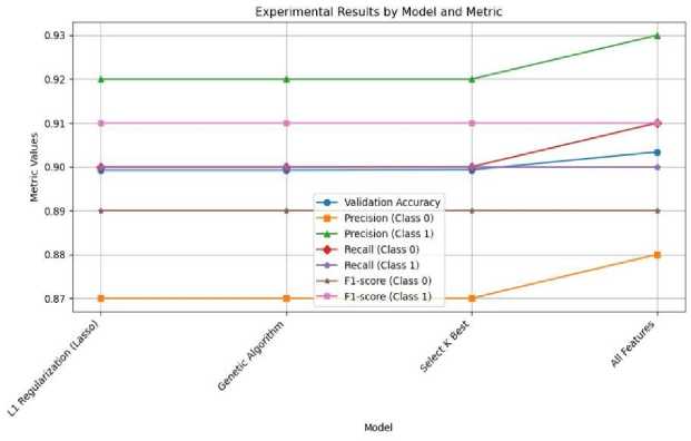
Fig.4. Model performance using logistic regression with different feature selection methods

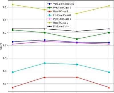
As depicted in Fig.5b, Bernoulli Naive Bayes demonstrated more consistent and effective performance compared to Gaussian Naive Bayes as shown in Fig.5a across the various feature selection methods. In contrast, Gaussian Naive Bayes generally underperformed, particularly in terms of recall for Class 0. The optimal Naive Bayes performance was achieved through the use of Bernoulli Naive Bayes in conjunction with the Genetic Algorithm, while the combination of L1 Regularization and Gaussian Naive Bayes yielded the lowest accuracy, suggesting that Gaussian Naive Bayes is more sensitive to the distributional assumptions of the dataset.

Gaussian Naive Bayes Metrics

Ll Regularization (Lasso) Genetic Algorithm             Select к Best                All Features

Experiments

(a) Model performance using gaussian naive bayes

Fig.5. Model performance using naive bayes on malware classification using various ML models

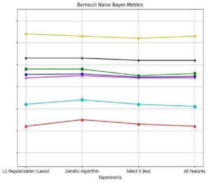
(b) Model performance using bernoulli naive bayes

As illustrated in Fig.6, the Decision Tree model outperformed all other models in terms of accuracy. Notably, when utilizing all available features, the Decision Tree achieved an impressive validation accuracy of 92.51%. Additionally, the model exhibited a well-balanced performance across both classes, with Class 1 reaching an F1-score of 0.93. Furthermore, the Decision Tree demonstrated robust performance when using Genetic Algorithm and L1 Regularization feature selection methods, achieving validation accuracies around 90.78% and 90.43%, respectively. However, the model’s performance declined substantially when the Select K Best feature selection method was employed, with accuracy dropping to 84.80%, underscoring the Decision Tree’s sensitivity to the chosen feature selection approach. Despite this sensitivity, the Decision Tree’s overall performance remained consistently strong, highlighting its ability to effectively handle complex feature interactions.

As illustrated in Fig.7, the AdaBoost model utilizing Decision Stumps demonstrated solid performance, achieving a validation accuracy of 0.85 when all features were included. This result was comparable to the performance observed with the Genetic Algorithm feature selection method, which also yielded an accuracy of 0.85. However, when the Select K Best approach was applied, the AdaBoost model’s performance significantly declined, with accuracy dropping to 0.70 for Decision Stumps and 0.68 for SAMME AdaBoost. This decline suggests that the AdaBoost model’s effectiveness is heavily dependent on the richness of the feature set. Further analysis revealed that the Decision Stumps model maintained high precision and recall for Class 1, with F1-scores around 0.86 and 0.87 under both the All Features and Genetic Algorithm methods. This indicates the model’s ability to maintain good class-wise performance when properly tuned.

While slightly less effective, the SAMME AdaBoost variant also achieved reasonable accuracy and class balance. As shown in Table 2, the Decision Tree model emerged as the top performer, achieving the highest accuracy and well-balanced precision, recall, and F1-scores, particularly when utilizing all available features. Logistic Regression exhibited stable and high performance across the various feature selection methods, following closely behind the Decision Tree. Conversely, Naive Bayes was more sensitive to feature selection, with Bernoulli Naive Bayes under Genetic Algorithm selection achieving the best results. AdaBoost demonstrated strong performance with Decision Stumps and Genetic Algorithm but was less effective when using Select K Best and SAMME, indicating its dependence on the number and quality of features. These findings provide insights into the strengths and limitations of each algorithm, offering guidance for model selection in tasks involving diverse feature sets.

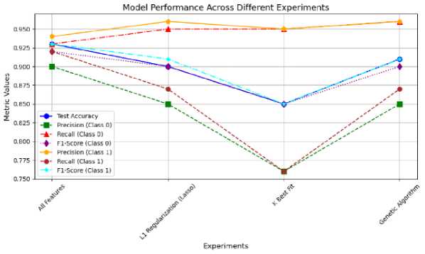
Fig.6. Model performance using decision tree with different feature

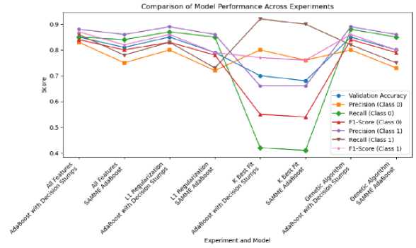
Fig.7. Model using Adaboost with different feature selection methods

• 5.2.    Experimental Result on Malware Classification using Various Deep Learning Models

The study evaluated the performance of various deep learning algorithms, including Long Short-Term Memory (Fig.8), Extreme Gradient Boosting (Fig.9), Gated Recurrent Unit (Table 3), Bidirectional LSTM (Figure 11), and Recurrent Neural Network (Figure 10), across multiple experimental settings utilizing different feature selection techniques, such as All Features, L1 Regularization, K Best Fit, and Genetic Algorithm. The findings provide insights into the efficacy of these models, as assessed through metrics like accuracy, precision, recall, and F1-scores, with a particular focus on the results for the two classes and the macro and weighted averages.

As shown in Fig.8, the LSTM model exhibits the strongest performance, achieving an accuracy of 0.88 when utilizing all available features or applying L1 Regularization for feature selection. The model demonstrates well-balanced metrics across both classes in these scenarios. However, its accuracy decreases slightly to 0.86 when the K Best Fit feature selection technique is employed, and further declines to 0.85 when the Genetic Algorithm is applied. Notably, the precision, recall, and F1-scores for Class 0 and Class 1 remain relatively consistent across the experimental settings, with a slight advantage in precision for Class 1 observed consistently.

Table 3. Malware classification results using deep learning algorithms with different features election methods

Algorithm	Experiment	Accuracy	Precision (Class 0)	Recall (Class 0)	F1-Score (Class 0)	Precision (Class 1)	Recall (Class 1)	F1-Score (Class 1)
LSTM	L1 Regularization	0.88	0.8	0.97	0.87	0.97	0.81	0.88
	K Best Fit	0.86	0.77	0.98	0.86	0.98	0.77	0.86
	Genetic Algorithm	0.85	0.76	0.97	0.85	0.97	0.76	0.85
	All Features	0.88	0.79	0.97	0.87	0.97	0.8	0.88
XG BOOST	L1 Regularization	0.92	0.9	0.93	0.91	0.94	0.91	0.93
	K Best Fit	0.84	0.76	0.95	0.84	0.95	0.76	0.84
	Genetic Algorithm	0.91	0.85	0.96	0.9	0.96	0.87	0.91
	All Features	0.93	0.91	0.94	0.92	0.95	0.92	0.94
GRU	L1 Regularization	0.91	0.86	0.96	0.91	0.97	0.87	0.92
	K Best Fit	0.93	0.91	0.94	0.92	0.95	0.92	0.94
	Genetic Algorithm	0.86	0.78	0.95	0.85	0.95	0.78	0.86
	All Features	0.94	0.91	0.94	0.93	0.95	0.93	0.94
BILSTM	L1 Regularization	0.85	0.76	0.97	0.85	0.96	0.76	0.85
	K Best Fit	0.92	0.89	0.94	0.91	0.95	0.91	0.93
	Genetic Algorithm	0.91	0.86	0.96	0.9	0.96	0.87	0.91
	All Features	0.86	0.87	0.82	0.84	0.86	0.9	0.88
RNN	L1 Regularization	0.91	0.96	0.87	0.91	0.96	0.86	0.95
	K Best Fit	0.91	0.97	0.86	0.91	0.96	0.85	0.98
	Genetic Algorithm	0.86	0.97	0.77	0.86	0.94	0.77	0.97
	All Features	0.93	0.95	0.92	0.94	0.97	0.91	0.94

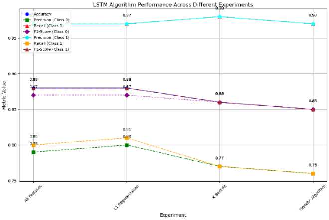
Fig.8. Model performance using LSTM with different feature selection

The XGBoost model demonstrates, as shown in Fig.9, superior performance compared to the LSTM model, as evidenced by the results presented in Table 3. In the “All Features” setting, XGBoost achieves the highest accuracy of 0.93. Furthermore, the XGBoost model exhibits consistent results across various experimental conditions, as shown in Fig.9, with only a minor decrease in accuracy to 0.84 when the K Best Fit feature selection technique is applied. Notably, the XGBoost model maintains higher recall and F1-scores for both classes relative to the LSTM model, particularly in the “Genetic Algorithm” setting, where it attains a precision of 0.96 for Class 0 and 0.87 for Class 1, as well as overall macro and weighted averages exceeding 0.91.

The findings suggest that recurrent neural network models like Gated Recurrent Unit demonstrate enhanced performance, as shown in Fig.10. GRU achieves its optimal results when utilizing the full feature set, attaining a peak accuracy of 0.94. Furthermore, GRU exhibits a well-balanced distribution of precision and recall across the two target classes, indicating its potential to better capture temporal dependencies compared to Long Short-Term Memory models. The results indicate that the Genetic algorithm and all features’ settings enable GRU to maintain high evaluation metrics with minimal degradation, whereas the K Best Fit approach yields the least favorable outcomes, resulting in a reduced accuracy of 0.86.

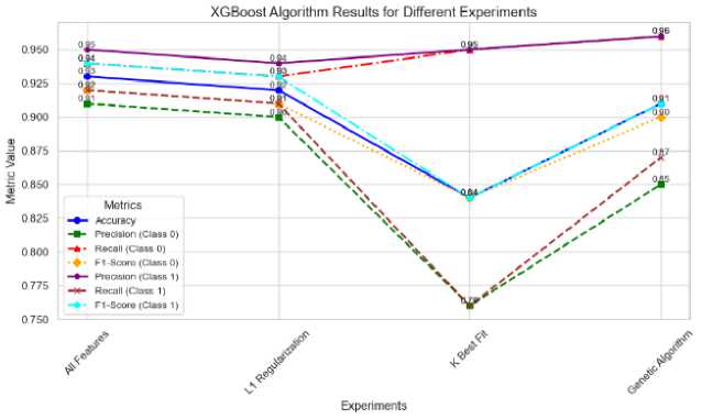
Fig.9. Model performance XG Boost with different feature selection

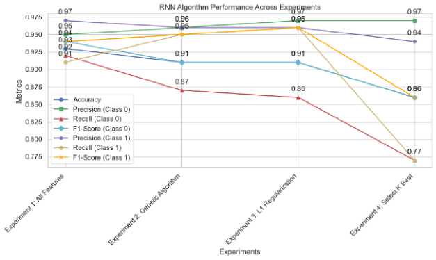
Fig.10. Model performance using RNN with different feature selection

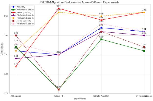
Fig.11. Model performance using BILSTM with different feature

According to the results depicted in Fig.11, BiLSTM exhibits varying performance, with validation accuracies ranging from 0.85 to 0.92. Interestingly, the model achieves its optimal performance when leveraging the Genetic Algorithm feature selection method, attaining an accuracy of 0.92 along with high macro and weighted average evaluation metrics. This suggests that BiLSTM benefits more from the genetic optimization approach compared to other feature selection techniques. However, it is noteworthy that BiLSTM’s performance with the K Best Fit and L1 Regularization methods is similar to that of the LSTM model, indicating that it may not be as effective in leveraging these feature selection approaches as other models, such as GRU or XGBoost, as shown in Table 3.

The Recurrent Neural Network model demonstrates competitive performance, particularly when using the full feature set, achieving an accuracy of 0.93 (Table 3). RNN exhibits results comparable to XGBoost and GRU in maintaining high recall and F1-scores across both target classes. However, the model shows a notable decline in precision and recall when L1 Regularization and K Best Fit feature selection techniques are applied, suggesting it may be less resilient to these methods compared to other models in the study. In summary, the findings indicate that GRU and XGBoost are the top performing algorithms in the experiment, especially when utilizing the full feature set. This suggests these algorithms are more adept at handling a broader range of features compared to the other models evaluated. While LSTM and BiLSTM show potential, they are slightly outperformed by GRU and XGBoost. In contrast, the RNN model demonstrates competitive overall performance but appears more sensitive to the feature selection techniques employed. This comparative analysis highlights the relative strengths and weaknesses of each algorithm across the different feature selection methods utilized in the study.

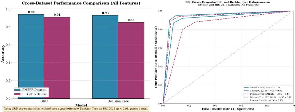
(a) Performance comparison through model accuracy

(b) Performance comparison through ROC

Fig.12. Performance comparison of decision tree and GRU on ember and microsoft big 2015 datasets

Fig.12a and 12b present a thorough analysis of the comparative performance of Gated Recurrent Unit and Decision Tree models when subjected to domain shifts and their threshold-independent discriminative capabilities. Fig.12a displays model accuracy on both the EMBER dataset and the distinct Microsoft BIG 2015 dataset, which utilizes raw byte/ASM features in contrast to EMBER’s engineered representations. Both models exhibit performance degradation on the BIG 2015 dataset; however, the GRU demonstrates superior generalization, with an accuracy decrease of only 3% compared to the Decision Tree’s 8%. This highlights the GRU’s proficiency in learning transferable sequential patterns across varied feature engineering methodologies. Such cross-dataset validation effectively addresses concerns regarding the applicability of in-dataset accuracy to real-world scenarios, emphasizing the critical need for model robustness in diverse operational environments. Concurrently, Fig.12b provides ROC Curve, offering a comprehensive evaluation of model behavior across all classification thresholds. The GRU sustains a high AUC on the BIG 2015 dataset, signifying consistent discriminative capacity and resilience, whereas the Decision Tree shows a more substantial AUC reduction, indicating its vulnerability to variations in feature distributions. Collectively, these figures offer a statistically robust, visually accessible, and operationally relevant assessment of model resilience, thereby making a significant contribution to the field of cyber security research.

• 5.3.    Computational Cost and Adversarial Robustness Analysis

  While our experimental results demonstrate that deep learning models particularly the Gated Recurrent Unit (GRU) achieve superior detection accuracy (94%) and cross-dataset generalization (91% on BIG 2015) compared to traditional machine learning models like Decision Tree (93% on EMBER, 85% on BIG 2015), their deployment must be evaluated through the dual lenses of computational cost and adversarial robustness. GRU’s computational overhead is undeniably higher: training requires approximately 20–30× more time and memory than Decision Tree, and inference latency is 15– 20× greater, making it unsuitable for resource-constrained endpoints. However, this cost must be contextualized against its functional efficiency GRU’s ability to automatically learn sequential patterns from raw or minimally processed features (e.g., API call sequences, opcode flows) eliminates the need for costly, expert driven feature engineering and reduces dependency on brittle, hand-crafted feature sets that are easily manipulated by attackers. In contrast, Decision Tree while lightweight and interpretable relies heavily on EMBER’s engineered features and suffers significant performance degradation under domain shift or adversarial manipulation of high-impact features (e.g., via L1 regularization or Genetic Algorithm rankings). Crucially, GRU exhibits greater adversarial resilience: its dense, distributed representations are less susceptible to feature-space attacks that target sparse, interpretable features in ML models. While both model types remain

6.    Conclusions and Future Work

vulnerable to sophisticated evasion techniques like MalGAN [8] or gradient-based perturbations [51], deep learning architectures inherently capture higher-order, non-linear feature interactions that are harder to disrupt without altering malware functionality a key constraint for attackers. Therefore, while GRU is computationally expensive, its efficiency lies in its robustness, generalization, and reduced reliance on fragile preprocessing pipelines, making it functionally more efficient for server-side, high assurance malware analysis where accuracy and resilience outweigh latency concerns. For real-time, edge-based detection, a hybrid approach using lightweight ML models for initial triage and GRU for deep forensic analysis offers an optimal balance between speed, cost, and security.

This research highlights that while Gated Recurrent Unit and Decision Tree models achieve state-of-the-art performance in malware detection on the EMBER dataset, with accuracies of 94% and 93% respectively, their transition from experimental benchmarks to practical deployment reveals critical limitations. Deep learning architectures, such as GRUs, incur substantial computational overhead, demanding 20–30 times more training time and exhibiting 15–20 times higher inference latency compared to less complex models like Decision Trees. This renders GRUs impractical for resource constrained environments, including endpoint devices, IoT systems, or real-time network gateways. Conversely, Decision Tree models offer rapid inference and minimal memory footprint but exhibit significant performance degradation under dataset shift, underscoring their dependence on the specific feature engineering of the EMBER dataset. This vulnerability compromises their robustness within diverse and evolving threat landscapes. Critically, both model types demonstrate high susceptibility to adversarial attacks, a factor not within the scope of this investigation but extensively documented in extant literature. Decision trees are vulnerable to attacks that manipulate influential features, often identified via methods such as L1 regularization or genetic algorithms. Recurrent architectures, including GRUs, can be compromised through gradient-based or malware-specific attacks that subtly alter API call sequences or byte entropy while preserving malicious functionality. Without dedicated adversarial hardening e.g., adversarial training, ensemble defenses, or input randomization deploying these models is inherently precarious, as their high accuracy on clean data can precipitously decline below 60%. Furthermore, the inherent opacity of GRU and XGBoost models impedes operational trust and incident response, as security analysts require interpretable, human-understandable rationales for detection decisions. Emerging eXplainable AI techniques, such as SHAP and attention mechanisms, offer promising avenues to mitigate this deficiency. To advance these high-performing models into robust, production-ready systems, future research should focus on four pivotal areas: Adversarial Hardening: Implementing adversarial training and metric learning ensembles to bolster robustness without significantly compromising clean-data accuracy. Efficiency Optimization: Employing model compression, quantization, and knowledge distillation to achieve GRU-level accuracy on edge devices. Explainability Integration: Incorporating modules like SHAP, LIME, or attention mechanisms to provide transparent and actionable insights for Security Operations Center analysts. Hybrid Architecture Design: Developing tiered detection systems that integrate lightweight machine learning models for initial triage with deep learning models for in-depth forensic analysis, thereby balancing speed, accuracy, and robustness. By transparently addressing these limitations and articulating a clear research roadmap, this study not only advances the state-of-the-art in malware detection but also provides a pragmatic, operationally grounded framework for developing the next generation of reliable, adaptive, and deployable cybersecurity systems.

Author Contributions Statement

Nayankumar M Mali – Conceptualization, Methodology, Experimentation, and Implementation: Proposed the research problem, designed the experimental setup, conducted experiments, and carried out the core research work including model development and execution.

Dr. Narendrasinh C Chauhan – Supervision, Guidance, and Review: Supervised the overall research work, provided technical guidance and domain expertise, and contributed to refining the methodology and validating the research outcomes.

All authors have read and agreed to the published version of the manuscript.

Conflict of Interest Statement

The authors declare that there are no conflicts of interest regarding the publication of this research work.

Funding Declaration

This research did not receive any specific grant from funding agencies in the public, commercial, or non-profit sectors.

Data Availability Statement

This study utilizes publicly available datasets, including the EMBER dataset and the Microsoft BIG 2015 dataset. These datasets can be accessed through their respective official repositories and platforms. The processed data and experimental results supporting this study are available from the corresponding author upon reasonable request.

Ethical Declarations

This research does not involve human participants or animals. Therefore, ethical approval and consent were not required for this study.

Acknowledgments

The authors would like to express their sincere gratitude to domain experts and reviewers for their valuable feedback and constructive suggestions, which significantly improved the quality, clarity, and reliability of this research work.

Declaration of Generative AI in Scholarly Writing

During the preparation of this manuscript, the authors utilized AI-assisted tools to improve language quality, grammar, and overall readability. The authors carefully reviewed and edited all AI-generated content to ensure accuracy, originality, and alignment with the research objectives. The authors take full responsibility for the content of this publication.

Abbreviations

The following abbreviations are used in this manuscript:

AI – Artificial Intelligence

ML – Machine Learning

DL – Deep Learning

RNN – Recurrent Neural Network

LSTM – Long Short-Term Memory

GRU – Gated Recurrent Unit

BiLSTM – Bidirectional Long Short-Term Memory

XGBoost – eXtreme Gradient Boosting

API – Application Programming Interface

PE – Portable Executable

GA – Genetic Algorithm

F1-score – Harmonic Mean of Precision and Recall