Aerial Video Processing for Land Use and Land Cover Mapping

Unmanned Aerial Vehicles (UAV) are playing increasingly prominent role in urban planning [1], agricultural analysis [2][3][4], environmental monitoring [5][6], traffic surveillance [7], texture classification [8] due to their low cost and safe operation as compared to manned aircrafts. The data is acquired using a video sensor and is in digital format which makes it very feasible to process. Earlier work has been done to differentiate buildings from other terrain [9][10], roof top detection using aerial images [11], road extraction from aerial images [12][13], and shadow detection in aerial images [14]. Color image segmentation [15], which quantizes the color into several representing classes, is often used to extract information about buildings from aerial images. However, automatic detection of buildings in monocular aerial images without elevation information is hard. Buildings cannot be easily identified efficiently using color information because they don’t have any characteristic RGB values unlike barren land or vegetation. Another approach employing Active Contour Model (ACM) or Snake model [16] has been used for automatic building boundary extraction but due radiometric characteristics of the building being same to image background some buildings were not extracted. A rapid man-made object segmentation based on watershed algorithm has been developed that creates homogenous regions [17]. So we propose a system for identifying man-made, vegetation and barren land features from the given aerial video.

In this paper, we have proposed a system for identification, extraction and classification of objects from the given aerial video. As is shown in Figure 3. initially, the aerial images are affected by radial distortion so we use fish-eye algorithm to reduce the distortions. The radial distortion free images are aligned and stitched using Scale Invariant Feature Transform (SIFT) and Random Sample Consensus (RANSAC) techniques. Stitched images are segmented by Mean Shift Segmentation method to extract Vegetation, manmade structures and Barren Land surface features. The extracted features are evaluated using ground truth data for evaluating the segmentation performance. The accuracy of the results is very efficient. The advantages of the developed system over the other existing methods are easy, efficient and robustness for video processing and instantaneous automatic object recognition. We have successfully classified three entities viz. Man-made structures, Vegetation, Barren land with an overall accuracy of 94%.

• II.    Study Area

The study field is shown in Figure 1. The Indian Institute of Science located in Bangalore (13°01'35N, 77°33'56E). The Institute spreads over 400 acres of land situated in the heart of Bangalore city. The institute is covered with different variety of trees and it is located at an altitude of about 920mtrs above sea level.

The UAV is flown above the study area and video is acquired. The acquired aerial video is about 3 minutes. From the acquired video five different image frames of the same area are extracted for our study.

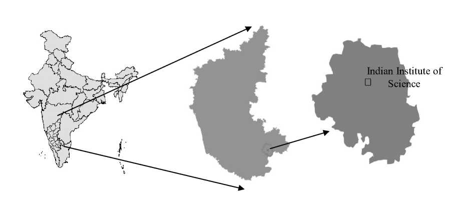
Figure 1. Study Area

• III.    Data Acquisition

  In this section, the description of aerial video acquired from the UAV plane is discussed. UAV is designed with the specifications as shown in the Table 1. The designed UAV is shown in the Figure 2. The aerial video camera is mounted under the UAV plane and aerial video is recorded. The flying altitude of UAV while acquiring data is 1030mtrs above sea level and image resolution obtained is about 3 cm per pixel. The UAV that we have used is a medium altitude surveillance vehicle. The UAV and camera specifications are given in Table 1.

• IV.    Methodology

In this section, we are discussing methods of aerial video processing system. The system is divided into three major steps: 1) Pre-Processing 2) Image registration and 3) Image segmentation.

• A.    Pre-Processing

The camera used to capture the land surface features consist of fisheye lenses which causes radial distortions in images. Correction of this video is called “Rectification of radial distortions” using fisheye correction[18] Fish-eye lenses have greater “field of view (FOV)” which in turn covers the greater area but leads to the cylindrical distortion.

Table 1. Specifications

UAV Specifications		Camera Specifications
Wing span	120Cm (Wing Span = 120cm , Wing Chord 17cm)	Camera Name	HD-PRO Camera with field of view 1700
Length	87 cms
Payload Weight	1.1Kg Total 1Kg (module weight) + 120grams( payload)	Video HD Resolutions	1080p: 1920×1080, 30 Frames per second (FPS)
Engine	Electronic type Myn is Brushless DC motor [1000Kv out runner]
Fuel tank:	It runs with battery [3cell LiPo, 2200Mah]	Field Of View(FOV)	Wide 170º FOV, Medium 127º FOV
Flight time:	10 minutes
Propeller:	9 x 4.7E

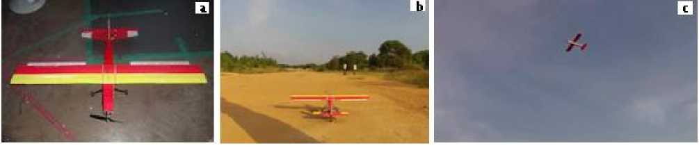
Figure 2. a) UAV designed for aerial video surveillance, b) UAV while takeoff and c) UAV while flying

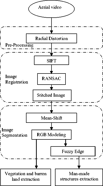
Figure 3. System Overview

The Corrected images from radial distortion is shown in Figure 5. Let x and y be the x and y coordinates respectively, of a target pixel in the output rectilinear perspective image, and similarly, let x and y be those of a source pixel in the input fisheye image. Let R (as shown in Figure 4.) be the radial position of a point in fisheye image and R is the radial position of a point in perspective image. Then assuming equisolid angle mapping for fisheye image, the below equations hold true.

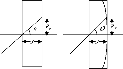
Figure 4. Projection of Non-fisheye and Projection of fisheye camera

R = 2 f sin( ^ /2)

Rp = f tan(^)

xpxf ypyf

2 x_p sin(tan - 1 ( 2 /2))

2 y sin(tan 1 ( 2 /2)) y f = —   2----

2 = (7 X p ² + y, ²)/ f

image _ width f = 4sin(FOVhorz /2)

• B.    Image Registration

In this step the radial distortion corrected images are aligned, transformed and stitched. Firstly, image features are found and matched with the features of the other image using SIFT and after that applying RANSAC to reduce the number of outliers and finally the image is stitched.

• 1)    Image Registration

The SIFT algorithm was proposed by David G. Lowe [19] operates in four major stages to detect and describe local features, or key points, in an image: a) Scale-space extrema detection, b) Key point localization, c)

Orientation assignment and, d) Key point descriptor. For image matching and recognition, SIFT features are first extracted from a set of reference images and stored in a database. A new image is matched by individually comparing each feature from the new image to this previous database and finding candidate matching features based on Euclidean distance of their feature vectors. Using Scale Space Function, we can detect the locations that are scale and orientation invariant. It has been shown by Koenderink [20] and Lindeberg [21] that under a variety of reasonable assumptions the only possible scale-space kernel is the Gaussian function.

The scale space (8) of an image is defined as a function, L ( x , y , k a ) , that is produced from the convolution of a variable-scale Gaussian, G ( x , y , a ) ,with an input image, I ( x , y ) .

L ( x , y , k a ) = G ( x , y , k a ) 0 1 ( x , y ) (8)

G ( x , y , a ) = -1y e "^{( x} 2 ⁺ y 2^{)2 a} 2 (9) 2na

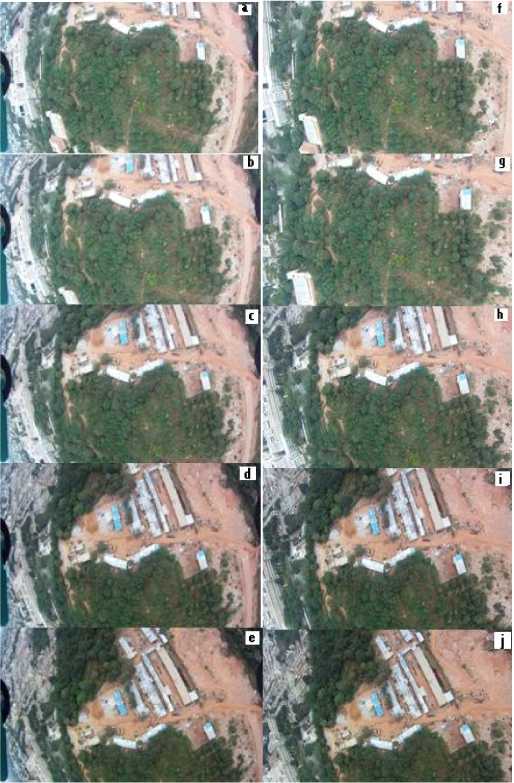
Figure 5. Five Image frames (a-e) are read from the given aerial video are corrected for radial distortion by using fish-eye correction algorithm which is shown in figure (f-j)

convolved with the image, D ( x , y , a ) can be used to detect the stable key point location in the sample space.

D ( x , y , a ) = L ( x , y , k,.a ) - L ( x , y , j )    (10)

Hence a DOG of an image between scales kza and kja   is just the difference of the Gaussian-blurred images at scales (10). In order to detect the local maxima and minima of D(x, y, a) , each sample point is compared to its eight neighbors in the current image and nine neighbors in the scale above and below. It is selected only if it is larger than all of these neighbors or smaller than all of them. By assigning a consistent orientation to each key point based on local image properties, the key point descriptor can be represented relative to this orientation and therefore achieve invariance to image rotation. The scale of the key point is used to select the Gaussian smoothed image, L , with the closest scale, so that all computations are performed in a scale-invariant manner. For each image sample, L(x, y) , at this scale, the gradient magnitude, m(x, y) , and orientation, 0(x, y) , is pre computed using pixel differences.

m ( x , y ) = ^( L ( x + 1, y ) - L ( x - 1, y ))² + ( L ( x , y + 1) - L ( x , y - 1))²   (11)

^ ( x , y ) = tan

^л L ( x , y + 1) - L ( x , y - 1) ^л _v L ( x + 1, y ) - L ( x - 1, y ) _v

After we get N Matched pairs, the RANSAC [22] robust estimation is used in computing 2D homography. The Random Sample Consensus (RANSAC) algorithm is a resampling technique that generates candidate solutions by using the minimum number observations (data points) required to estimate the underlying model. The parameters for N iterations where N is number of matched pairs:

Select randomly the minimum number of points required to determine the model parameters.

Solve for the parameters of the model.

Determine how many points from the set of all points fit with a predefined tolerance.

s over the total number points in the set exceeds a predefined threshold, reestimate the model parameters using all the identified inliers and terminate.

Procedure:

Let u represent the probability that any selected data point is inliers.

Let v = 1 - u the probability of observing an outlier. N iterations of the minimum number of point’s denoted m are required, where

The Difference-of-Gaussian (DOG) function

mN

1 — p = (1 — u )

and thus with some manipulation,

_N= log ^{(1 —} p )

log(1 — (1 — v )")

In stitching one important step that is involved is image warping (Figure 6.). It is merging of several images into a complete 2D mosaic image. In Stitching the transformation between images is often not known beforehand. In this example, two images are merged and we will estimate the transformation by letting the RANSAC matched pairs of correspondence in each of the images

Let X = [x y 1] denote a position in the original 2D image I and X' = [ x' y' 1] denote the corresponding position in the warped image I ,

" x '"		5 COS	s sin	Tx"		■ x"
t y	=	— ssin	s cos	Ty	X	y	(15)
_ 1 _		_   0	0	1 _		_ 1 _

Where s is the scaling factor, Tx and Ty are the horizontal and vertical translations respectively and α is the rotation angle. Here, since we are dealing with the Aerial images we should warp the whole image about 4 points. This transformation is called perspective transformation. So replace X and X' by x1

X =

X ' =

y 1 1

x 1' y 1' 1

x2

y2

x 4 y 4 1

x2'   x3'

y2'   y3'

The Transformation matrix denoted by T is

X ' = T * X

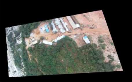
Figure 6. Warped Image

Finally the aerial images are stitched by applying the proposed algorithm recursively for frames extracted sequentially from the video. The final step of stitching is to project the input images onto a common 2D coordinate system .The warped images are projected with respect to a reference frame. To apply the proposed algorithm for video, first two images are warped by applying perspective transformation for the second image with respect to first image and stitched on the 2D coordinate system. Then the third image is warped with respect to second image and so on. The final stitched image is shown in Figure 7.

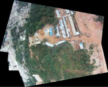
Figure 7. Stitched Image

• C.    Image Segmentation

Image segmentation is the process of partitioning an image into multiple segments. The goal of segmentation is to simplify and/or change the representation of an image into something that is more meaningful and easier to analyze. Image segmentation is typically used to locate objects and boundaries in images. More precisely, image segmentation is the process of assigning a label to every pixel in an image such that pixels with the same label share certain visual characteristics. There are various techniques for image segmentation based on different approaches. In this paper we have employed Mean Shift Segmentation and Fuzzy Edge Detection.

• 1)    Image Segmentation

Mean Shift [23] is a robust and non-parametric iterative algorithm. For each data point, Mean shift associates it with the nearby peak of the dataset’s probability density function. For each data point, mean shift defines a window around it and computes the mean of the data point. Then it shifts the center of the window to the mean and repeats the algorithm till it converges. After each iteration, we can consider that the window shifts to a denser region of the dataset. After all the iterations we get final mean shift segmented image as shown in Figure 8.

Let a kernel function K ( x_f — x ) be given. This function determines the weight of nearby points for reestimation of the mean. Typically we use the Gaussian kernel on the distance to the current estimate.

K ( x_t - x ) = e cxi - x l2

The weighted mean of the density in the window determined by K is:

. .   2 x G N ( x ) K ( x, - x ) x

=--- iii

2 x_t g N ( x ) K ( x _;. - x )

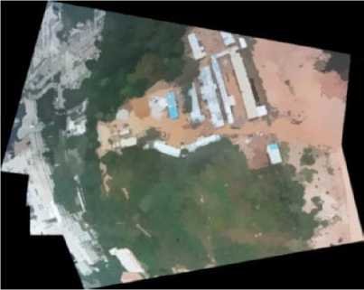
Figure 8 Mean Shift Segmentation

Where N ( x ) is the neighborhood of , a set of points for which K ( x ) ^ 0 . The mean-shift algorithm now sets m ( x ) ^ x , and repeats the estimation until converges.

• 2)    RGB Model

The RGB color model is an additive color model in which red, green, and blue light are added together in various ways to reproduce a broad array of the name of the model comes from the initials of the three additive primary colors, red, green, and blue. So on the basis of values of R, B and G different terrains and structures are distinguished.

Here, we use the fact that each type of terrain has a unique set of RGB values and we differentiate objects on the basis of their respective RGB values. For example vegetation will have a set of RGB values corresponding to green and barren land would have different set of RGB values.

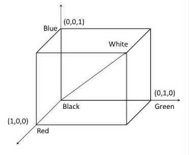
Figure 9. RGB Color Space

• 3)    Fuzzy Edge Detection

We can use RGB values to identify vegetation or barren land because of their characteristic values but in the detection of Man-Made structures we can’t have specific RGB values. So we have incorporated a hybrid model to identify man-made structures employing Fuzzy Inference Ruled by Else-Action (FIRE), Else-Action (FIRE), designed by Russo and Ramponi [24] with RGB Model.

f = max( f 1,...., f 8)

An input image has luminance values [250] from {0, 1… 255}. For pixel P , let

W j    ^{{ P}( i - e )( j - f ) ,...., P ( i + e )( j + f )^}

where e , f G |_ 0,... K / 2 J and K is the window size, be the set of pixels in the neighborhood of P with the exception of P (hence, | W y |= K * K - 1 ).

The inputs to the fuzzy edge extractor are the luminance differences between pixels in W to P ,

x,._ =w... X-P                       (23)

( ij , m )         ( ij , m )        ij                                             ( )

1 <  m <  ( K * K - 1)

th

Where W(ij,m) is the mt element in the window centered at P .

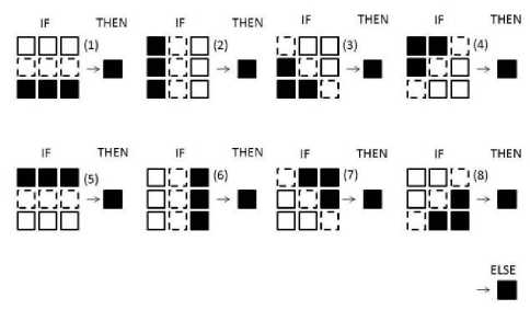
Figure 10. The eight rules in the fuzzy rule base.

All subsequent operations performed on X are independent of all other pixels, therefore, X will be notationally reduced to X , to simplify the indexing and as all discussion is about a specific P and its W . The domain of is the set {- 255, . . , 255}.

A simplified rule is : If a pixel lies upon an edge, then make it black Else make it white.

Eight unique cases (Figure 10), representing an edge at every 45 degrees of rotation, figure is represented as a rule. Each rule has six antecedents, coinciding with six of the eight pixels in X. Fuzzy sets are used to represent the linguistic terms negative and positive. Similarly, the linguistic uncertainties of the consequent terms white and black are also modeled as fuzzy sets.

For each pixel, each of the eight rules consisting of six antecedents are fired using the values in X. For each rule, the average of the six confidences is used as the total antecedent firing f , where 1 ≤ i ≤ 8 . In this algorithm, it is assumed that a given pixel can belong to, at most, one of the eight cases. Therefore, the rule with the largest firing f is used as the antecedent firing strength to the fuzzy consequent set representing black.

And in addition to that we have set a threshold to detect edges of Man-Made structures only i.e. f if is greater than threshold then only edge of man-made structures will be detected.

• V.    Results And Discussions

The correction of radial distortion is important for efficient processing. Figure 5 shows radially distorted and corrected images. The corrected images are then matched and stitched using SIFT followed by RANSAC. The efficiency of the stitching depends on the number of matched features which comes out to be very good and RANSAC then reduces the number of outliers. The stitched image is then segmented using Mean-Shift Segmentation which is followed by RGB modeling for vegetation and barren land extraction. For man-made structures, we employ a hybrid method incorporating fuzzy edge detection with Mean Shift Segmentation. In Mean Shift Segmentation, the efficiency of the results depends on three parameters viz. radius of space variables named as spatial radius, radius of color variables called color radius and max-level which stands for the number of scale pyramid we want for segmentation. The optimum results are observed at spatial radius=10, circle radius=20 and max level=2. A shift from these values leads to decrease in efficiency of the results. The resulting segmented image using above stated parameters is shown in Figure 8. For Fuzzy edge detection, the threshold values which are the difference in luminescence value of two adjoining pixels are significant in determining the accuracy of the results. We set a threshold of 100 to achieve optimum results. In order to check the correctness of the system, we calculated the user accuracy and producer’s accuracy of the segmented images by comparing processed results with the ground truth data. The respective accuracy is shown in the table below for different segmented images also shown below in Figure 11. Furthermore, the overall accuracy of the system comes out to be 94.02% as shown in the Table 2. The inability of the system in achieving 100% accuracy is credited to different camera calibrations and flight angles during UAV flight. For better results, the nadir point of the camera must coincide with the principal point of the lens. But when UAV is inclined at a greater angle, then this condition is hard to satisfy and so there is loss in quality of the acquired images and hence loss in accuracy occurs. Moreover, the relative lack of accuracy in building extraction is due to the fact that unlike vegetation cover and barren land which have same RGB values, buildings have varying RGB values.

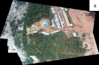
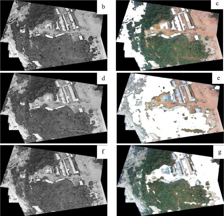
Figure 11. a) Stitched Image, b), d) and f) Contours drawn for Man-Made Structures, Vegetation and Barren Land respectively, c), e) and g) Area extracted (white regions) for Man-Made Structures, Vegetation and Barren Land respectively

Table 2. User Accuracy and Producer Accuracy of the proposed system by identifying and extracting different entities.

*data in pixels

Aerial Data
		Man-Made Structures	Vegetation	Barren	Other	Total	Producer Accuracy
	Man-Made Structures	107797*	5083	1547	2931	117358	91.85%
1 ts R to	Vegetation	5810	292625	589	0	299024	97.86%
	Barren	1615	428	142480	4388	148911	95.68%
	Other	3476	6494	2533	5468	17971	30.42%
	Total	118698	304630	147149	12787
	User Accuracy	90.81%	96.06%	96.83%	42.76%
						Overall Accuracy	94.02%

• VI.    Conclusions

The task of image stitching and image segmentation has been successfully accomplished by above discussed procedure. This method has been found to be an efficient and versatile approach for segmentation as we have applied it on different samples of images and compared the results. The system has shown high accuracy in vegetation and manmade structure classification and extraction. Considering that this is an instantaneous image processing system, the results are efficient. Although the methodology developed in this paper has been successfully applied but still some limitations were detected. The main limitations are related to flight angle and camera calibrations. This can be rectified by using a pre-defined path for UAV, so that a threshold inclination can be achieved beyond which processing of acquired image is not efficient.

Acknowledgment

This work is supported by the Space Technology Cell, Indian Institute of Science and Aeronautical Research and Developers board (ARDB). We thank the reviewers for his/her thorough reading and suggesting many important aspects. All the suggestion was very useful in revising our article.