Algorithm of Processing Navigation Information in Systems of Quadrotor Motion Control

Nowadays, numerous researchers all over the world pay attention to processing information in the quadrotor’s control systems. We can explain this fact by the permanently widening sphere of the quadrotor’s applications and by the vast variety of their flight missions, which became more and more complicated. On the other hand, the quadrotor is a very convenient testbed for the applications of the new approaches of modern control and information theories. Among the huge diversity of these approaches, we will pay attention to very popular methods of creating algorithms for processing information in control systems, for example, the linear-quadratic synthesis, which is successfully applied to the designing of the single quadrotors flight control algorithms [1 - 3], as well as in the cases of the quadrotor formations [4, 5]. One of the essential advantages of this approach is the simplicity of processing navigation information and obtaining of control algorithm based on the static state feedback consisting of the simplest static gains without any dynamic blocks. However, these methods require complete measurement of such navigation information as all components of the state vector of the mathematical model of the quadrotor. In many practical cases, this measurement is incomplete, because such a component of the state vector as the rotation rate of the quadrotor’s propeller is not measurable. That is why in these cases static output feedback is applied instead of static state feedback [6 – 8].

It is necessary to note, that in [7, 8] the method of the static output feedback synthesis is derived from the linear quadratic synthesis and can be considered as some extension of the linear quadratic synthesis. The main result of [7, 8] is the minimization of L -gain, which is the measure of the external disturbance suppression, which is very important for quadrotor flights in a turbulent atmosphere. This method was used for the static output feedback synthesis of the quadrotor flight control in cases when the quadrotor with its control system was considered a holonomic system [9], and a nonholonomic system as well [10]. It is necessary to note also, that in [11] the method was applied for control of the quadrotor formation flight.

All aforementioned results were obtained for continuous control systems. However, in practical cases, all real control systems are digital discrete control systems. It was supposed by default, that the sampling period is small enough for applying these results in the discrete case also. At the same time, the sampling periods in the real airborne microprocessors have finite values, which must be taken into account. Especially, it is important for executing the general procedure of unmanned aerial vehicles’ computer-aided design, which includes model-in-loop simulation, software-in-loop simulation, and hardware-in-loop simulation [12]. Two last cases require the usage of digital control algorithms and information processing for their execution. Another reason to consider discrete models of the quadrotor dynamics and control appears in the case of quadrotor usage in multi-agent formations. In this case, the information exchange between different agents leads to time delays, which negatively influence the stability of the single quadrotor as well as the stability of the whole formation [4, 5]. Therefore, the goal of this article is the creation of an algorithm for information processing using the application of the L -gain minimization method for the development of the discrete control algorithm for the quadrotor control system. Results obtained in [7, 8, 11] are based on the usage of the algebraic Riccati equation for continuous systems. However, the algebraic Riccati equation for the discrete systems differs essentially from the algebraic Riccati equation, therefore results of [7, 8] cannot be applied in this case.

That is why; we propose the minimization of L -gain using simple parametric optimization for the development of the algorithm for processing information in a digital control system based on static output feedback. The structure of this article includes the problem statement, a brief description of the linearized quadrotor model, the problem solution and the case study, and the simulation of the closed-loop control system with an extended model, which consists of the initial linearized model, used in the minimization procedure, augmented with some essential nonlinearities immanent to the real control plant.

2.    Problem Statement

In this article, we will consider a quadrotor as a rotorcraft with four propellers. Fig. 1 represents its kinematical diagram. In this aircraft, the front M₂ and back electric motors M₄, rotate counterclockwise. At the same time, lateral electric motors M 1 and M 3 rotate in the opposite direction. The united input represents the sum of thrusts of every motor 4

T = ∑ T . The pitch angle is changing as a result of the increasing (decreasing) rate of the back electric motor M₄ with i = 1

the simultaneous decreasing (increasing) rate of the front electric motor M 2 . The roll angle changes in a similar way using lateral electric motors M 1 and M 3 . Control of rotation around the vertical axis is realized by increasing (decreasing) rates of front and back motors with simultaneous decreasing (increasing) rates of lateral motors. These processes must be accompanied by keeping stable total thrust T z . In Figure 1, P is the radius vector of the quadrotor center, ψ , θ , ϕ are angles of yaw, pitch, and roll, respectively.

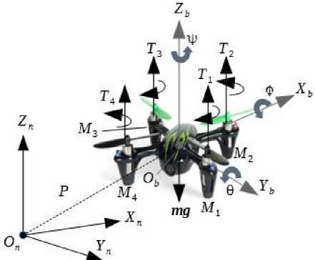
Fig. 1. The quadrotor kinematics diagram

We will consider the planar motion of the quadrotor for the Xn- and Yn- axes and the constant altitude Zn=const. Consider the decomposition of its spatial motion along 3 axes in the body frame (longitudinal Xb, lateral Yb, and vertical Zb). The symmetry of the quadrotor construction for these axes (see Fig. 1) substantiates this decomposition. Numerous publications, including [1, 4, 9, 10, 13], accept this assumption and represent the models of the quadrotor partial motions in the standard Cauchy form. Taking into account, that the models of motions for the Xn- and Yn-axes are identical [1, 4, 9, 10, 13], we will consider only the model of the motion along Yn-axis dX( t )= A x( t) + BuU (t)+ BwW(t),

u (t ) = C x( t), z (t) =

4Q  0 5 x 1   "Z( t )’

0 i x ₅    Rr JL ^{u (} t ) _ .

where: x , u, and z are the state, output, and desired output vectors, respectively. Vectors x and и include the following components

X = [X 1 ,X 2 ,X 3 ,X 4 ,Х 5Г = [ y , dy / ^dt ,Ф, P , ^{AQ ]} , и = [ y , dy / dt , ф, p ]^T.

In expression (2) y,dy dt are a position of a quadrotor on the Y -axis and its linear velocity along this axis, respectively; ф , p are roll angle and roll rate, and AQ is the increment of the rotation rate of the quadrotor’ motors, located on the Y -axis, which produces a control input u ( t ). Existing airborne equipment does not allow the AQ measurement in the majority of practical situations, therefore the application of the standard procedure of creating a linear quadratic regulator is not possible in this problem. In addition, it is necessary to mention that w ( t ) is the exogenous disturbance, which is the component of the turbulent wind velocity acting along the Y -axis. The numerical values of matrices A e R ^{5 x 5}, B_u e R ^{5 x 1}, B_d e R^{5 x 1}, C e R^{4 x 5} are presented in [9], and we will give them later in the “Problem Solution” and “Case Study” sections. Matrices Q and R are weighting matrices, and 0 i _{x 5}, 0_{5 x} i are zero matrices with corresponding dimensions.

One can easily transform the continuous system (1) into discrete form with a given sampling period т _s using standard procedures [14, 15] or simply applying the MATLAB command “c2d.m”. After this procedure, we obtain the system of difference equations in discrete time k

X ( ^{k +} 1 ) = A d x ( ^k ) ⁺ B Ud ^u ( ^k )⁺ B wd d ^{( k} ), ^u( ^k ) = ^C d x ( ^k ) ,

~ VQ  0 5 x 1 1Гх ( k ) !

z ( k ) =                         .

o_{1 x 5}   VR JL ^{u ( k} ) _

Here matrices Q and R define the quadratic cost function for the discrete system [14, 16, 17]

to                               to

J_c = ^ [ z ^T( k ) z ( k )] = £ [X^T( k ) U ^T( k )] k = 0                     k = 0

Q . 01 x 5

0 5 x 1   Гх( k )■

R JL u ( k )

Suppose that the closed-loop quadrotor control system with static output feedback as control algorithm is stable, and this static output feedback looks like

K y = [ K y , K dy / dt , K ф , K p ].

where K , K , K , K are static gains for corresponding variables of output υ in expression (2). Then the control input of the quadrotor model looks like u (k) = -KY u( k) = - K¥C x( k).

Figure 2 shows the generalized scheme of the closed-loop system for the quadrotor motion along with the Y -axis corresponding to the equations (1) and (6), where block “Quadrotor model” corresponds to the system (1).

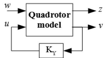
Fig. 2. The scheme of the control system for Y -axis motion.

Following [7, 8, 18], we introduce bounded L 2 - gain for discrete closed-loop system (1), (6), and any energy-bounded disturbance w ( k ) as follows

L 2 = _∞ ^Jc    ≤ γ ² .                                                  (7)

∑ w ²( k ) k = 0

The problem lies in finding such a gain of static output feedback K∈ R1×4 that satisfies inequality (7) for a closed-loop system. Note that the minimal possible value of γ in (7) is denoted as γ*, so γ > γ* . In this case, the static output feedback, which satisfies [7, 19], is called H -output feedback [7, 8]. The necessary conditions for its existence are the following: the pairs of matrices (A, Q) (A,C) must be detectable, and the pair (A,B) must be stabilizable [7, 8]. As was mentioned above, the method of such feedback synthesis was developed in [7, 8] for continuous systems (1). In a ∞ discrete system, we propose to minimize (7) by K , K , K , K static gains, under assumptions that ∑w2 (k) = 1 , k=0

and closed-loop system (1), (6) remains stable during the execution of the L -minimization procedure. Therefore, we can formulate the problem statement as follows

Find : K^* = argmin J ( K ) ; subject to: K^* ∈ D ,                              (8)

where admissible domain D determines the stability domain of system (1), (6) in the K ^* parameters space. We can define it as follows

E i = eig i (A - B u K Y^* C) ∈ D p , i = 1 ,..., 5 . ,                                       (9)

where eig ( A - B K^* C ) are eigenvalues of the state propagation matrix of the closed-loop system (1), (6), and D is the prescribed domain inside the unit circle of the complex plane. Its violation produces a penalty function (PF), which restricts the procedure of the minimum searching by domain D . We will determine it in the next item.

• 3.    Problem Solution

Let W ( z ) is the transfer functions matrix between disturbance w and the state vector χ , and W ( z ) is the transfer function between w and control input u of the closed-loop system depicted in Fig. 2. Here z = e ^{j ωτ s} . Then the quadratic cost function for the closed-loop discrete system (4) we can express as follows [15, 20]

J c = ¹ ∫ tr[W w ^T χ ( z ^{- 1}) QW w χ ( z )] ^dz + ¹ ∫ W w ^T u ( z ^{- 1}) RW wu ( z ) ^dz ,                        (10)

2 π j _Λ z   2 π j _Λ z

The symbol Λ in (10) denotes the unit circle in the complex plane. From the computational point of view, expression (10) we can rewrite in the following form [15, 21, 22]

J_c =[ H 2 ( 4Q ■ W w x ( z )) ] 2 +[ H 2 ( 4R ■ W wu ( z )) ] ²,

where H ₂ ( - )are the H ₂ -norms of the corresponding transfer functions.

Now we have to define the admissible domain D in the expression (9) for pole placement of the closed-loop system during the execution of the minimization procedure. Figure 3 depicts this domain inside the unit circle of the complex plane.

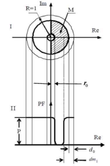
Fig. 3. The pole placement of the admissible domain D p : PF – penalty function.

Figure 3 shows the domain D of the PF definition inside the unit circle (section I) and PF profile (section II), represented as its cross-section through the real axis Re [16]. D is determined by the following restrictions: the semicircle with the larger radius 1 - d_Q , which defines the stability margin d ₀, and the semicircle with the smaller radius r , which defines the maximal frequency band. The domain d is shown in Fig. 3 as a shaded region. Let E_m ( k ) = max_j(abs( E ( k ))) at the current k th iteration of the minimization procedure. Define the distance d_m ( k ) = 1 - E_m ( k ) . Then the expression for penalty function PF will have the following form

0if d m ^ d m 1 ,

PF 1 (d m )= ^

P

PF 1 ( d m )= ^P

P if d m ^ d 0 -

' 1 + cos H ^d m — ^d 0) I

( ^(d m 1 — ^d 0 )

^{if d} 0 >  ^d m >  ^d m 1 , ’

where P is a large value ( P =10⁴-10⁶).

PF ₁ is defined as a violation of the area bounded by the larger radius 1 - d . A similar penalty function PF ₂ is defined for the smaller radius r , so the total penalty function equals PF = PF 1 + PF 2 . Eventually, we can define the minimized total cost function as follows

J. = [ H 2 ( 4Q ■ W w x ( z ))] 2 + [ H 2 (V R ■ W w„ ( z ))] 2 + PF .

Now we will illustrate the application of the parametric synthesis of the control law with the L -gain minimization for the real quadrotor [23, 24].

A certain disadvantage of the control algorithm (8), (4) is the necessity to find the initial value of the static output feedback gain matrix K ( 0 ) defined in (5), which guarantees the stability of the closed-loop system (3), (6), i.e. satisfying condition (9) [19, 20]. This disadvantage is absent for the continuous system [7, 8, 21]. However, it is possible to find the “hint about the answer” after the solution of the discreet algebraic Riccati equation and command “dlqr.m” for the system (3), assuming that all state variables x = [ У , dy I dt , Ф , P , AQ ]^T are observable.

4.    Case Study

Consider the quadrotor, which was developed and manufactured at the National Aviation University (Kyiv, Ukraine). Its mathematical model in the form (1) is described in [9]. The matrices A, B , B , C for the model of the quadrotor motion along Y_n -axis (Fig.1) have the following numerical values [9]

	"0     1       0    0     0  "
			"1   0  0  0  0"
	0   - 0.28  9.81  0    0
			01000
A =	0    0     0    1    0	, C =		\                       (14)
			0 0 10 0
	0    0     0   0  0.22
			_ 0  0  0   1   0 _
	_ 0    0      0   0   - 8.33 _
B w =	[ 0  1  0   - 6.72  0 ] T , Bu =	[ 0  0	0  0  664.3 ] T .

The onboard microprocessor EPSON for control system implementation provides a sampling frequency 125 Hz (sampling period t_s = 0 . 008 sec). Executing MATLAB command “c2d” with this sampling period, we receive the following matrices of the discrete state-space model

	"1	8 - 10 - 3	3 - 10 - 4		0	0    "
	0	0.9978	0.0784	3	10 - 4	0
A d =	0	0	1	8	10 - 3	0	,,                                            (15)
	0	0	0		1	1.7 - 10 - 3
	_ 0	0	0		0	0.9355 _

B wd = [0 , 8 - 10 - 3 , - 2 - 10 — 4 , - 0 . 0571 , 0]^T , B ud = [0 , 0 , 0 , 4 . 6 - 10 ^{- 3} , 5 . 1412]^T ,  C d = C.

Define the weighting matrices Q and R in the cost function (4) for the solution of the standard DLQR problem as follows

Q = diag {[10, 10, 20, 20, 1]}; R =1.

Solving the problem of creating the standard discrete linear quadratic regulator with matrices A ,B ,Q,R from (15), (16), we obtain the initial value of the static output feedback gain matrix for starting the minimization procedure (8), (9)

K (0) = [0 . 584 , 0 . 9715 , 8 . 3241 , 3 . 8796 , 0 . 1791] .

After neglecting the last gain for the unobserved variable AQ and executing the optimization procedure with weighting matrices Q =diag{[10, 10, 20, 20]}and R =1, we obtain the following static output feedback gain matrix

K * = [0 . 5581 , 1 . 5492 , 2 . 1659 , 2 . 0835] .

The eigenvalues (9) for the closed-loop system corresponding static output feedback gain (18) have the following values

E_t = {0 . 9668 ± j 0 . 13 , 0 . 9965 ± j 0 . 0217 , 0 . 9971},

Considering the input disturbance w ( t )) having unit H -norm, we obtain the estimation of γ ² in (7) as γ ² = J^min = 0 . 578, i.e. γ = 0 . 76 . Note, that due to the [7, 8] the necessity and the sufficiency of the H -norm of static output feedback gain existence is proved by the usage of the following weighting matrix Q = C^T C , which in our case is the unit matrix. That is why, it is important to estimate the norms of the transfer function matrix W ( e^{j ωτ s} ), which show actual suppression of the disturbance w ( t ) without any weighting functions. They have the following values H ( W ( e ^{j ωτ s} )) = 0 . 1051 , H ( W ( e ^{j ωτ s} )) = 0 . 1852 . The first value can be considered as the γ ^* value, so γ > γ ^* , and K^* from (18) can be considered as H of static output feedback gain [7,8]. These estimations prove the efficiency of the disturbance suppression.

The synthesis of the H static output feedback gain for the control algorithm of the quadrotor motion along the X -axis is absolutely the same as in the previous situation, besides only one correction. In matrix A , appearing in (14), it is necessary to change only the sign of the A (2,3) entry: A (2,3)=-9.81 [1, 13, 17, 23, 24]. Taking into account this circumstance and repeating exactly the previous procedure of synthesis, we will obtain the following matrix of the static output feedback gains for the X -axis as follows

K^* = [ - 0 . 5581 , - 1 . 5492 , 2 . 1659 , 2 . 0835] . (20)

All numerical characteristics presented above are the same as in the previous situation. It would be useful to mention, that in this situation, state vector will have the form: % = [ x, dx / dt, 0, q, A^ ] T , where x is the quadrotor position on X -axis, θ , q are the pitch angle and pitch rate, respectively.

5.    Simulation of the Quadrotor Guidance in the Turbulent Atmosphere

Atmospheric conditions [25-27] including turbulence [28, 29] affect significantly any aircraft flight control. The intensity of atmospheric turbulence, which according to ICAO is normally measured by eddy dissipation rate (EDR) [30], is not the only important characteristic to estimate the influence onto aerial vehicle. Another important parameter is the turbulence scale [31]. It is well known that the smaller is a flight vehicle the smaller turbulent whirls affect its behavior during flight [32]. There are developed methods of simulation taking into account both indicated parameters [33, 34]. However, these methods are rather complicated. They are important for modeling relationships between turbulence and information signals for estimating turbulence characteristics using, for example, coherent polarimetric radar [35, 36]. In case of our task, we can use a simplified approach just using the root mean square (rms) of turbulence, which actually depends on both EDR and turbulence scale, as the only parameter of turbulence.

The simulation of the quadrotor guidance in the Simulink package is necessary for further estimating the usefulness of the proposed control algorithms. To make simulation conditions closer to operating flight conditions as much as possible, we augment the linear models of the quadrotor dynamics (14) with some initial nonlinear elements linearized for the synthesis procedure. Consider the model of the quadrotor planar motion, which follows from [13, 37 -40]

_d 2 _x dt ² d ² y dt ²

µ dx    tan θ

• -      - g     ,

m dt   cos ϕ

µ dy

• -      - g tan ϕ .

m dt

In system (21), µ and m are the drag force coefficient [18, 20, 21, 39, 40] and the total mass of the quadrotor, respectively. We have used this system (21) instead of (14) for the closer approximation of the operating flight conditions with the simulation conditions, and for estimations of the linearization errors based on the simulation results. We have also included the saturation elements at the inputs of actuators (electrical motors) because they are obligatory for quadrotor flight safety. Figure 4 shows the block diagram of the simulated system. In this figure, RTG is the reference track generator (in our case, it is the circular track), M , M are the mathematical models of X and Y subsystems (21), K , K are the SOF gain matrices (18), (20), ZOH are zero-order holds. Also, it is necessary to mention that X , Y are the reference values for the quadrotor’s position, while X , Y are the values of the quadrotor actual position. The link ϕ between M , M reflects the presence of this variable in the first equation of the system (21). At last, D , D are the series connections of the white noise generators and Dryden filters, generating the models of the longitudinal and lateral components of the turbulent wind velocity vector [19, 41 - 43]. We have chosen the root mean square (rms) of these components to be commensurable with the cruise velocity of the heavy quadrotor (6 -7 m/sec).

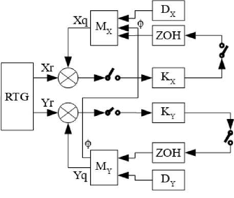
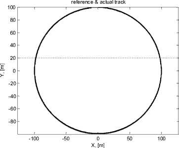
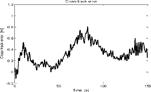
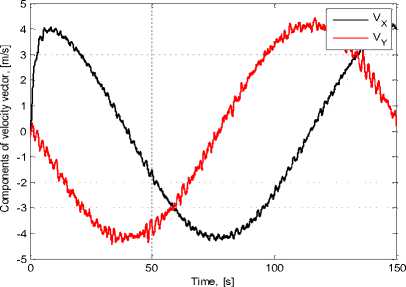
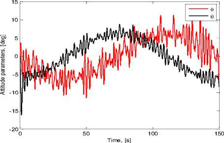
Figure 5 presents the simulation results. As it is possible to see from Fig. 5a and Fig. 5b, the cross-track error of the control system is sufficiently small.

Fig. 4. The diagram of the simulated system

(а)

(b)

(c)

(d)

Fig. 5. Results of the quadrotor guidance simulation: a) reference track (black), actual flight path (grey); b) cross-track error; c) components of the velocity vector: V x - (black), V y - (grey); d) pitch angle (black), roll angle (grey).

Its mean value equals 0.328 m, and the centered error equals 0.176 m. Taking into account that the reference track radius is 100 m; we can state that the accuracy of the control system is good. On the other hand, Fig. 5d shows that the maximum value of the pitch angle equals 15o (or 0.26 rad) during a very small time, meanwhile during the whole time of tracking the pitch and roll angles do not exceed 10o (or 0.17 rad).

The substitutions cos ϕ≈ 1 and tan θ ≈ θ for the linearization of the system (21) produce errors of 0.015 and 0.006 respectively. Therefore, the linearization of (21) is justified, as well as the application of the aforementioned method of control law synthesis [44, 45].

6.    Conclusion and Future Research Directions

The algorithms for processing information in discrete control systems for the quadrotors have been considered in this article. The developed algorithms have been implemented in the real onboard equipment. It has been shown that some of the state vector components, like increments of the propeller’s rotation rates, are unobservable in the onboard measurement equipment, and this should be taken into account. This circumstance requires applying the static output feedback synthesis of the quadrotor control algorithm because the static output feedback is the simplest control algorithm implemented in the onboard microcontroller.

The most appropriate procedure for this algorithm creation is the minimization of the L -gain of the closed-loop system. As far as this procedure without search was developed for continuous systems [6 - 9, 46 - 49], we developed the procedure of the parametric synthesis (3) for the discrete system if all state variables % = [ У, dy / dt, Ф , P, A^ ] T are observable.

The obtained results can be also useful for tests of unmanned aerial vehicles [50 - 52] and the design of airborne stabilization systems [53, 54].

Future research directions are associated with improving processing navigation information based on filtering; using the loop-shaping approach for the synthesis of control algorithms; studying the possibility to improve the control algorithm based on the method of the mixed sensitivity.

Acknowledgment

We would like to express our gratitude to the reviewers for their precise and succinct recommendations that improved the presentation of the results obtained.

Conflict of Interest

The authors declare no conflict of interest.