Algorithmic representation of the quantum operators and fast quantum algorithms

Author: Barchatova Irina, Hagiwara Tahiko, Ulyanov Sergey
Journal: Сетевое научное издание «Системный анализ в науке и образовании» @journal-sanse
Article in issue: 3, 2014.
Free access
The simplest technique for simulating a quantum algorithm (QA) is described and is based on the direct matrix representation of the quantum operators. This approach is stable and precise, but it requires allocation of operator’s matrices in the computer’s memory. Since the size of the operators grows exponentially, this approach is useful for simulation of QAs with a relatively small number of qubits (e.g., approximately 11 qubits on a typical desktop computer). Using this approach it is relatively simple to simulate the operation of a QA and to perform fidelity analysis. Two special search algorithms: Shor’s and Grover’s QA are described.
Quantum operators, fast quantum algorithms, аlgorithmic representation
Short address: https://sciup.org/14122611
IDR: 14122611
Алгоритмическое представление квантовых операторов и квантовых алгоритмов
Описана простая техника моделирования квантового алгоритма, основанная на прямом матричном представлении квантовых операторов. Такой подход является устойчивым и точным, но требует огромного объема оперативной памяти компьютера для вычисления матричного представления квантовых операторов. Так как простарнственно-временная размерность операторов возрастает экпоненциально, то такой подход может быть использован для моделирования квантовых алгоритмов с относительно малым числом входных кубитов (т.е. примерно 11 кубитов для типовой конфигурации ПК). Используя этот подход, можно моделировать относительно просто квановые алгоритмы и достигать высокого качества результата. Даны примеры моделирования двух поисковых квантовых алгоритмов: алгоритм Шора и алгоритм Гровера.
Text of the scientific article Algorithmic representation of the quantum operators and fast quantum algorithms
In one embodiment, a more efficient fast QA simulation technique is based on computing all or part of the operator matrices on an as needed current computational basis. Using this technique, it is possible to avoid storing all or part of the operator matrices. In this case, the number of qubits that can be simulated (e.g., the number of input qubits, or the number of qubits in the system state register) is affected by: (i) the exponential growth in the number of operations required to calculate the result of the matrix products; and (ii) the size of the state vector that is allocated in computer memory.
In one embodiment, using this approach it is reasonable to simulate up to 19 or more qubits on typical desktop computer, and even more on a system with vector architecture.
Due to particularities of the memory addressing and access processes in a typical desktop computer (such as, for example, a Pentium-based Personal Computer), when the number of qubits is relatively small, the compute-on-demand approach tends to be faster than the direct storage approach. The compute-on-demand approach benefits from a study of the quantum operators, and their structure so that the matrix elements can be computed more efficiently.
The study portion of the compute-on-demand approach can, for some QAs lead to a problem-oriented approach based on the QA structure and state vector behavior [1 – 3].
For example, in Grover’s quantum search algorithm (QSA), the state vector always has one of the two different values: (i) one value corresponds to the probability amplitude of the answer; and (ii) the second value corresponds to the probability amplitude of the rest of the state vector. Using this assumption, it is possible to configure the algorithm using these two different values, and to efficiently simulate Grover’s QSA.
In this case, the primary limit is a representation of the floating-point numbers used to simulate the actual values of the probability amplitudes. After the superposition operation, these probability amplitudes are very small ( ).
2 n
Thus, it is possible to simulate Grover’s QSA with this approach simulating 1024 qubits or more without termination condition calculation and up to 64 qubits or more with termination condition estimation based on Shannon entropy.
Other QAs do not necessarily reduce to just two values. For those algorithms that reduce to a finite number of values, the techniques used to simplify the Gover’s QSA can be used, but the maximum number of input qubits that can be simulated will tend to be smaller, because the probability amplitudes of other algorithms have relatively more complicated distributions. Introduction of an external excitation can decrease the possible number of qubits for some algorithms.
In some algorithms, the entanglement and interference operators can be bypassed (or simplified), and the output computed based only on a superposition of the initial states (and deconstructive interference of the final output patterns) representing the state of the designed schedule of control gains. For example, a particular case of Deutsch-Jozsa’s and Simon algorithms can be made entanglement free by using pseudo-pure quantum states.
The disclosure that follows begins with a comparative analysis of the temporal complexity of several representative QAs. That analysis is followed by an introduction of the generalized approach in QA simulation and algorithmic representation of quantum operators. Subsequent portions describe the structure representation of the QAs applicable to low level programming on classical computer (PC), generalizations of the approaches and introduction of the general QA simulation tool based on fast problem-oriented QAs.
The simulation techniques are then applied to a quantum control algorithm.
The matrix-based approach can be efficiently realized for a small number of input qubits. The matrix approach is used above as a useful tool to illustrate complexity issues associated with QA simulation on classical computer.
1. Structure of QA gate system design
As shown in Fig. 1 (a), a QA simulation can be represented as a generalized representation of a QA as a set of sequentially-applied smaller quantum gates. From the structural point of view, each QA is based on a particular set of quantum gates, but generally speaking each particular set can be divided into superposition operators, entanglement operators, and interference operators.
This division into superposition operators, entanglement operators, and interference operators permits a generalization of the design of a simulation and allows creation of a classical tool to simulate QAs. Moreover, local optimization of QA components according to specific hardware realization makes it possible to develop appropriate hardware accelerators for QA simulation using classical gates.
|
Repeated k times |
||||
|
1 H |
||||
|
U F |
||||
|
|0> n |
—► ___________________________ 1 |
|||
|
.. . 1—► H |
||||
|
|0> |
||||
|
S |
||||
|
|x> m |
—► ___________________________ 1 |
|||
|
.. . 1 1 i 1 |
||||
|
|x> |
||||
|
Input |
Superposition Entanglem |
|||
|
. . . . . . |
|||||
|
—I—► —I—► —I-- I I |
INT |
I I I I --u I I I —I--H I I I |
h ► bit h .. . —► bit h bit |
M E A S U R E M E N T |
|
|
I I |
—► |
||||
|
I I I I I I |
h. . . |
||||
|
it I________________________________________________________________________I ___________________________________________________ ent Interference Output |
|||||
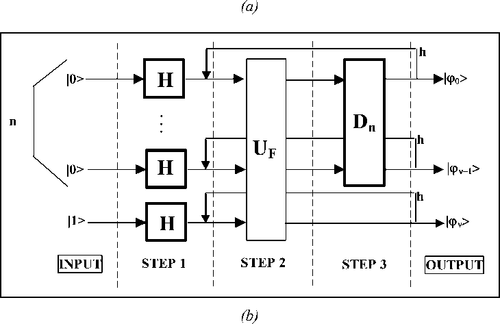
Figure 1. (a) Circuit representation of QA; (b) Quantum circuit of Grover’s QSA
2. Generalized approach in QA simulation
In general, any QA can be represented as a circuit of smaller quantum gates as shown in Figs 1 (a, b). The circuit shown in the Fig. 1 (a) is divided into five general layers: (i) input; (ii) superposition; (iii) entanglement; (iv) interference; and (v) output.
Layer 1: Input. The quantum state vector is set up to an initial value for this concrete algorithm. For example, input for Grover’s QSA is a quantum state | ^ ) described as a tensor product
|^ ) = a |0)®-.®|0) ®|0) + a 2|0)®-.®|0)® Ц + a 3|0)®-® Ц®|0) +••• + a Ц ®-® Ц ® 11 = 1|0> ®-®| 0) ® 11 = |0-01),
where |0) =
Г 1

; ® denotes Kronecker tensor product operation.
Such a quantum state can be presented as shown on the Fig. 2 (a).
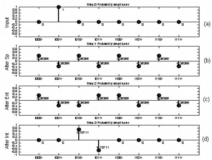
Figure 2. Dynamics of Grover’s QSA probability amplitudes of state vector on each algorithm step
The coefficients a in the Eq. (1) are called probability amplitudes. Probability amplitudes can take negative and/or complex values. However, the probability amplitudes must obey the following constraint:
Z a 2 = 1.
i
The actual probability of the arbitrary quantum state ai to be measured is calculated as a square of its probability amplitude value pi = | ai |2.
Layer 2: Superposition . The state of the quantum state vector is transformed by the Walsh-Hadamard operator so that probabilities are distributed uniformly among all basis states. The result of the superposition layer of Grover’s QSA is shown in Fig. 2 (b) as a probability amplitude representation, and also in Fig. 3 (b) as a probability representation.
Layer 3: Entanglement . Probability amplitudes of the basis vector corresponding to the current problem are flipped while rest basis vectors left unchanged. Entanglement is typically provided by controlled-NOT
(CNOT) operations. Figures 2 (c) and 3 (c) show results of entanglement from the application of the operator to the state vector after superposition operation. An entanglement operation does not affect the probability of the state vector to be measured. Rather, entanglement prepares a state, which cannot be represented as a tensor product of simpler state vectors. For example, consider state ф shown in the Fig. 2 (b) and state ф presented on the Fig. 2 (c):
ф = 0.35355(| 000) -1 001) + 1010> -| 011) + 1100) - |101) + 1110) - |111) )
= 0.35355(| 00) +1 01) +1 10) + 111) ) (| 0) -1 1) )
ф = 0.35355(| 000) -1 001) - 1010) + | 011) + 1100) - 1101) + 1110) - 1111) )
= 0.35355 (| 00) - 101) + 110) + 111) )| 0) - 0.35355 ( 00) + 101) + 110) + 111) )| 1)
As shown above, the description of state ф can be presented as a tensor product of simpler states, while state ф (in the measurement basis {|0),|1)}) cannot.
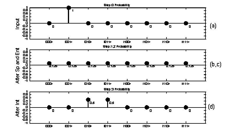
Figure 3. Dynamics of Grover’s QSA probabilities of state vector on each algorithm step
Layer 4: Interference . Probability amplitudes are inverted about the average value. As a result, the probability amplitude of states «marked» by entanglement operation will increase.
Figs 2 (d) and 3 (d) show the results of interference operator application.
Fig. 2 (d) shows probability amplitudes and Fig. 3 (d) shows probabilities.
Layer 5: Output . The output layer provides the measurement operation (extraction of the state with maximum probability), followed by interpretation of the result. For example, in the case of Grover’s QSA, the required index is coded in the first n bits of the measured basis vector.
Since the various layer of the QA are realized by unitary quantum operators, simulation of quantum operators depends on simulation of such unitary operators. Thus, in order to develop an efficient, simulation, it is useful to understand the nature of the QAs basic quantum operators.
3. Basic QA operators
The superposition, entanglement and interference operators are now considered from the simulation viewpoint. In this case, the superposition operators and the interference operators have more complicated structure and differ from algorithm to algorithm. Thus, it is first useful to consider the entanglement operators, since they have a similar structure for all QAs, and differ only by the function being analyzed.
In general, the superposition operator is based on the combination of the tensor products Hadamard
H operators: H = -^=
- 1
with identity operator I : I =
Remark. The simulation system of quantum computation is based on quantum algorithm gates (QAG). The design process of QAG includes the matrix design form of three quantum operators: superposition (Sp) , entanglement ( U ) and interference (Int) . In general form, the structure of a QAG can be described as follows:
QAG = [(Int ®n I)• UF] h+1 •[nH® m S], where I is the identity operator; the symbol ® denotes the tensor product; S is equal to I or H and dependent on the problem description. One portion of the design process in QAG is the type-choice of the entanglement problem-dependent operator U that physically describes the qualitative properties of the function f .
The Hadamard Transform creates the superposition on classical states, and quantum operators such as CNOT create robust entangled states. The Quantum Fast Fourier Transform (QFFT) produces interference.
For most QAs the superposition operator can be expressed as
Sp = ®H |®|® S | , (3)
I i = 1 ) X i = 1 )
where n and m are the numbers of inputs and of outputs respectively. The operator S depends on the algorithm and can be either the Hadamard operator H or the identity operator I . The numbers of outputs m as well as structures of the corresponding superposition and interference operators are presented in Table 1 for different QAs.
Table 1.Parameters of superposition and interference operators of main quantum algorithms
|
Algorithm |
Superposition |
m |
Interference |
|
Deutsch’s |
H ® I |
1 |
H ® H |
|
Deutsch-Jozsa’s |
nH ® H |
1 |
nH ® I |
|
Grover’s |
nH ® H |
1 |
D n ® I |
|
Simon’s |
nH ® nI |
n |
nH ® nI |
|
Shor’s |
nH ® nI |
n |
QFT n ® nI |
Superposition and interference operators are often constructed as tensor powers of the Hadamard operator, which is called the Walsh-Hadamard operator. Elements of the Walsh-Hadamard operator can be obtained as
• j
1 f ( n - 1) H
2 n '2
( n - 1) H
( n - 1) H )
- ( n - 1) H J ,
where i = 0,1, j = 0,1, H denotes Hadamard matrix of order 2.
The rule in Eq. (4) provides way to speed up of the classical simulation of the Walsh-Hadamard operators, because the elements of the operator can be obtained by the simple replication described in Eq. (4) from the elements of the n - 1 H order operator. For example, consider the superposition operator of Deutsch’s algorithm n = 1, m = 1, S = I :
[ SP ]
Deutsch i. j
= ( - 1 ) i*j 0 I = ' f ( - 1) 0*0 1
2 1'2 72 X ( - 1) 1*0 1
( - 1) 0*1 1) 1 Г I I
( - 1) 1*1 1 J = 72 [ I - 1
As a further example, consider the superposition operator of Deutsch-Jozsa’s and of Grover’s algorithm, for the case n = 2, m = 1, S = H :
^^-^j Deutsch - Jozsa ' s , Grover ' s 2 ^ ^) JJ
1 13H _
Vs J H =
H 2 H I 1
' H H
Vs ( 2 H - 2 H J Vs H
, H
H
- H
H
- H
H
H
- H
- H
H ) - H
- H
H ,
•
For yet another example, the superposition operator n = 2, m = 2, S = I can be expressed as:
of Simon’s
and
of Shor’s algorithms
Г о 1 Simon , Shor
[ Sp J i,j
, 1 f ( - 1) 0*0 H
H 0 I =
2 ( ( - 1) 1*0 H
( - 1) 1*0 H
( - 1) 1*1 H
2 1 =
1 ( H
H I
2 V H - H
0 2 1 =
|
f 1 |
1 |
1 |
1 1 |
' ’ I |
2 I |
2 I |
||
|
1 |
1 |
- 1 |
1 |
- 1 |
0 2 I = 1 |
' I |
- 2 I |
2 I |
|
2 |
1 V 1 |
1 - 1 |
- 1 - 1 |
- 1 1 J |
2 |
’ I V 2 1 |
2 I - 2 I |
- 2 I - 2 I |
- 2 1
- 2 1
Interference operators are calculated for each algorithm according to the parameters listed in Table 1. The interference operator is based on the interference layer of the algorithm, which is different for various algorithms, and from the measurement layer, which is the same or similar for most algorithms and includes the m th -tensor power of the identity operator.
The interference operator of Deutsch’s algorithm includes the tensor product of two Hadamard transformations, and can be calculated using Eq. (4) with n = 2 as:
L Int
Deutsch
i .. j
^1 1 11
2 _ (-1) i*j _1 f (-1)0*0 H (-1)0*1 H) 1 1 -1 1
H = 22/2 = 2 V (-1)1*0 H (-1)1*1 H J = 2 1 1 -1
1 -1 -1
In Deutsch’s algorithm, the Walsh-Hadamard transformation in the interference operator is used also for the measurement basis.
The interference operator of Deutsch-Jozsa’s algorithm includes the tensor product of the n th power of the Walsh-Hadamard operator with an identity operator. In general form, the block matrix of the interference operator of Deutsch-Jozsa’s algorithm can be written as from the n -1 order matrix as:
1 f (n-^H (n-1)H I (11
Г Int Deutsch - Jozsa ' s 1 = n H 0 I = 0 I , where H =
L J 2n/2 Vn-1) H -n-1) Hj ’V
Interference operator of Deutsch-Jozsa’s algorithm n = 2, m = 1:
I 1 1
I-
-1-
- II
Г Int Deutsch - Jozsa's 1= 2 h 0 1 = 1 1 H H I0 1 = 1
L J 2 V h -h J
The interference operator of Grover’s algorithm can be written as a block matrix of the following form:
Г Int
Grover
i ,. j
= D „ 0 1 = | - n I |0 1 = 1- 1 + |0 1
n 12 n /2 ) I 2 n /2 )
-17 I®I 2 n/2 )
_ 1 [- 1 , i = j
. . “ 2 n /2 1 I , i * j ’ i * j
where i = 0,...,2 n — 1, j = 0,...,2 n — 1 , Dn refers to diffusion operator:
[ D - ] , „= —
1 AND ( i = j )
2 n /2
.
For example, the interference operator for Grover’s QSA, when n = 2, m = 1 is:
[ Int Grover
—
:I |®I = |—1 +1|®I
) I 2)
,
i = j
1 I® I 2 1
i * j
As the number of qubits increases, the gain coefficient will become smaller. The dimension of the matrix increases according to 2 n , but each element can be extracted using Eq. (9), without allocation of the entire operator matrix.
Remark . Since DnDn * = I , Dn is unitary and is therefore a possible quantum state transformation. While the matrix Dn is clearly unitary it can to have the decomposition form D„ = — Hn R 1 H„ , where R [ i , j ] = 0, if i * j , R 1 [ 1,1 ] = — 1 and R ^ [ i , i ] = + 1, if 1 < i < N .
In concrete form the operator D ( diffusion – inversion about average ) in Grover algorithm is decomposed as
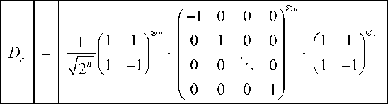
and can be accomplished with O ( n ) = O (log( N )) quantum gates. It means that from the viewpoint of efficient computation the form as in Eq. (9) is more preferable.
The interference operator of Simon’s algorithm is prepared in the same manner as the superposition (as well as superposition operators of Shor’s algorithm) and can be described as follows from Eq. (3) and Eq. (6):
( i * j )
Г I-t Simon 1 = n H ® m I = ( ) ( n - 1) h ® mJ
L J ( i , j ) 2 - /2
where H =
Л 1
I 1
—1,
In general, the interference operator of Simon’s algorithm coincides with the interference operator of Deutsch-Jozsa’s algorithm Eq. (8), but for each block of the operator matrix includes m tensor products of the identity operator.
The interference operator of Shor’s algorithm uses the Quantum Fourier Transformation operator (QFT), calculated as:
[ QFT n L ,
i J ( i * j )2 n = e 2
2 n /2 ,
where J = V- T , i = 0,...,2 n - 1 and, j = 0,...,2 n - 1 .
When n = 1 then:
QFT n
f ^ J *(0*0)2 п /2 1
2 2 V
j J *(1*0)2 п /21
J J *(0*1)2 п /21 ^
J *(1*1)2 п /21
e 2
V2 V 1
= h
-1)
Eq. (11) can also be presented in harmonic form using the Euler formula:
[ QFT ] = — cos l ( i * j) — | + J sin l ( i * j) — I
-
n ij n/2 nn
For some applications, the harmonic form of Eq. (13) is preferable.
General case. For most algorithms, the superposition operator can be expressed as: kA ,Lf kA .I
Sp = ® H ® ® S , where k, and L are the numbers of the inclusions of H and of S into the corre-V i=1 2 V i=1 2 12
sponding tensor products. Values of k , k depend on the concrete algorithm and can be obtained from Table 2.
Table 2. Parameters of superposition and of interference operators of QAs
|
Algorithm |
k 1 |
k |
S |
Interference |
|
Deutsch’s |
1 |
1 |
I |
H ® H |
|
Deutsch-Jozsa’s |
n - 1 |
1 |
H |
k1 H ® I |
|
Grover’s |
n - 1 |
1 |
H |
D k. ® I |
|
Simon’s |
n /2 |
n /2 |
I |
k1 H ® k 2 I |
|
Shor’s |
n /2 |
n /2 |
I |
QFTki ® k 2 I |
Operator S , depending on the algorithm, may be the Walsh-Hadamard operator H or the identity operator I . It is convenient to automate the process of the calculation of the tensor power of the Walsh-Hadamard operator as follows:
г -, (-1) 1 f1, if i * j is even
Г nH 1 = = ,(14)
L J •,j 2n/2 2n/2 [-1, if i * j is odd where i = 0,1,...,2n, j = 0,1,...,2n. The tensor power of the identity operator can be calculated as
ГnI 1i,j= 1I, =, 0|„„(15)
where i = 0,1,...,2 n , j = 0,1,...,2 n . Then any superposition operator can be presented as a block matrix of the following form:
(-1У+ j
[ Sp 1 i^yk)^ ®k 2 S •(16)
where i = 0,...,2k' -1, j = 0,...,2 k1 -1 denote the blocks; k 2 S is a k2 tensor power of the corresponding operator. In this case n denotes the total number of qubits in the algorithm, including measurement qubits, and qubits necessary for encoding of the function. The actual number of input bits in this case is k . The actual number of output bits in this case is k . Operators used as S are presented in the Table 2 for all typical models of QAs.
Let us consider examples.
For the superposition operator of Deutsch’s algorithm: n = 2, k = 1, k 2 = 1, S = I :
Deutsch
[ SP ] .
■. -
( - i ) ' +2 i Г ( - 1) 0*0 1
0 I =
2 1/2 V2 ( ( - i) 1*0 1
( - 1) 0*1 1) 1 Г I I
( - 1) 1*1 1 J = J' [ I - 1
The superposition operator of Deutsch-Jozsa’s and of Grover’s algorithm is,
n = 3, k = 2, k 2 = 1, S = H :
( - 1) 0*0 H
( - 1) 1*0 H
( - 1) 2*0 H
|
г -i Deutsch - Jozsa ' s , Grover [ Sp ] |
' s i ,. - ( - |
_ (- 1 ) 2 2/2 1) 0*3 H ) |
- 0 |
H = |
||||
|
( - 1) 0*1 H |
( - 1) 0*2 H |
Г H |
H |
H |
H ) |
|||
|
( - 1) 1*1 H |
( - 1) 1*2 H |
( - |
1) 1*3 H |
_ 1 |
H |
- H |
H |
- H |
|
( - 1) 2*1 H |
( - 1) 2*2 H |
( - |
1) 2*3 H |
2 |
H |
H |
- H |
- H |
|
( - 1) 3*1 H |
( - 1) 3*2 H |
( - |
1) 3*3 H J |
I H |
- H |
- H |
H J |
|
The superposition operator of Simon’s and of Shor’s algorithms are,
n = 4, k = 2, k 2 = 2, S = I :
[ Sp ] Simon ’ Shor^ ^(^т - ■ 1 ,
|
=1 |
Г ( - 1) 0*0 ( - 1) 1*0 |
( 2 1 ) ( 2 1 ) |
( - 1) 0,1 ( 2 1 ) ( - 1) 1*1 ( 2 1 ) |
( - 1) 0*2 ( - 1) 1*2 |
( 2 1 ) ( 2 1 ) |
( - 1) 0*3 ( - 1) 1*3 |
( 2 1 ) ) ( 2 1 ) |
_ 1 |
Г 2 I 2 |
2 1 - 2 1 |
I I 2 I - 2 I |
|
2 |
( - 1) 2*0 |
( 2 1 ) |
( - 1) 2,1 ( 2 1 ) |
( - 1) 2*2 |
( 2 1 ) |
( - 1) 2*3 |
( 2 1 ) |
2 |
2 1 |
2 1 |
- 2 1 - 2 1 |
|
. ( - 1) 3*0 |
( 2 1 ) |
( - 1) 3,1 ( 2 1 ) |
( - 1) 3*2 |
( 2 1 ) |
( - 1) 3*3 |
( 2 1 ) J |
1 2 1 |
- 2 1 |
-2 7 2 1 J |
The interference blocks implement the interference operator which, in general, is different for all algorithms. By contrast, the measurement part tends to be the same for most of the algorithms. The interference blocks compute the k tensor power of the identity operator.
Interference operator of Deutsch’s algorithm. This interference operator of Deutsch’s algorithm is a tensor product of two Walsh-Hadamard transformations, and can be calculated in general form using Eq. (14) with n = 2 :
|
Г 1 |
1 |
1 |
1 > |
|
|
Int D^ch 1 = 2 H = -Ц).- - = 1 |
1 |
- 1 |
1 |
- 1 |
|
J i,- 2 2/2 2 |
1 |
1 |
- 1 |
- 1 |
|
I 1 |
- 1 |
- 1 |
1 J |
Note that in Deutsch’s algorithm, the Walsh-Hadamard transformation in interference operator is used also for the measurement basis.
Interference operator of Deutsch-Jozsa’s algorithm. The interference operator of Deutsch-Jozsa’s algorithm is a tensor product of k power of the Walsh-Hadamard operator with an identity operator. In general form, the block matrix of the interference operator of Deutsch-Jozsa’s algorithm can be written as:
Г Int
Deutsch - Jozsa ' s
( -1Г '
k 1
0 I ,
|
^_Illt Deutsch - Jrzsa ' 5 J |
_ ( - ])- i , j 2 2 2 |
- ® I = |
|
|
< ( - 1) 0*0 1 |
( - 1) 0*1 1 ( - 1) 0*2 1 |
( - 1) 0*3 1" |
( I I I 1 1 |
|
( - 1) 1*0 1 |
( - 1) 1*1 1 ( - 1) 1*2 1 |
( - 1) 1*3 1 |
_ 1 I - 1 I - 1 |
|
( - 1) 2*0 1 |
( - 1) 2*1 1 ( - 1) 2*2 1 |
( - 1) 2*3 1 |
2 I I - 1 - 1 |
|
t ( - 1) 3*0 1 |
( - 1) 3*1 1 ( - 1) 3*2 1 |
( - 1) 3*3 1 ) |
t I - 1 - 1 I , |
•
Interference operator of Grover’s algorithm: The interference operator of Grover’s algorithm can be written as a block matrix of the following form:
ГIntGrove 1 = D, ®I = | -17 — k11 I®I = 1-1 + 4» I®I
L J i , j k 1 I 2 k i /2 J I 2 k i /2 у
| I®/
, I 2 ^ 1 /2 I
1 I - 1 , i = J
= I !,. - J' <23)
i * J V J
where i = 0,...,2 1 - 1, J = 0,...,2 k 1 - 1 , D^ refers to diffusion operator:

( - 1)
1 AND ( i = J )
2 k - 1
Thus, the interference operator of Grover’s algorithm for n = 3, kx = 2, k 2 = 1 is constructed as follows:
Г Int "rrv'
® I
i * J
—
|
J i , J = D 2^ |
' 12 2/2 |
J t 2 J |
|
|
1) |
1 |
1 |
1 |
|
- 1 +- I |
I |
I |
I |
|
2 1 |
2 |
2 |
2 |
|
1 |
( 0 |
1 |
1 |
|
I |
- 1+- I |
I |
I |
|
2 |
t 2 J |
2 |
2 |
|
1 |
1 |
1 |
|
|
I |
I |
- 1+- I |
I |
|
2 |
2 |
t 2 J |
2 |
|
1 r |
1 r |
, 1 |
|
|
I |
I |
I |
-1 + - |
|
2 |
2 |
2 |
2 |
, 1 2
® I
i * J
Note that as the number of qubits increases the gain coefficient becomes smaller and the dimension of the matrix increases according to 2 k 1 . However, each element can be extracted using Eq. (23), without constructing the entire operator matrix.
Interference operator of Simon’s algorithm The interference operator of Simon’s algorithm is prepared in the same manner as the superposition operators of Shor’s and of Simon’s algorithms and can be described as follows (see Eqs. (16), (19)):

(-1Y * j k H ®k 2 I = v ’ ® k 21
2 k 1 /2
( - 1) 0*0 - k 2 1
1 2^ 2
( - 1) i *0 - k 2 1
( - 1) 0* J - k 2 I ••• ( - 1) 0* ( 2 k 1 - 1 ) - k 2 I
( - 1) ‘ *J - k ' 2 I - ( - 2 k 1 - 1 ) - k 2 1
t ( - 1) ( 2 k - 1 ) 10 - k 2 1
( - 1) ( 2 k 1 - J k 2 I . (- 1) ( 2 k 1 - 1H2 k 1 - 1 ) - k 2 I
In general, the interference operator of Simon’s algorithm is similar to the interference operator of Deutsch-Jozsa’s algorithm Eq. (21), but each block of the operator matrix Eq. (25) is a k tensor product of the identity operator.
Each odd block (when the product of the indexes is an odd number) of the Simon’s interference operator Eq. (25), has a negative sign. Actually if i = 0,2,4,...2 k 1 - 2 or j = 0,2,4,...2 k 1 - 2 the block sign is positive, otherwise the block sign is negative. This rule is applicable also for Eq. (21) of the Deutsch-Jozsa’s algorithm interference operator.
Then it is convenient to check if one of the indexes is an even number instead of calculating the product. Thus Eq. (25) can be reduced as:
Inf- 1 = k H ® ‘ 2- I - (-^ ® f = 4т ( k 2 1 • if i is odd or if j is odd .
J i , j 2k 1 2k 1 [- k 2 1 , if i is even and j is even
Interference operator of Shor’s algorithm. The interference operator of Shor’s algorithm uses the Quantum Fourier Transformation operator (QFT), calculated as:

- 1 J k1 Ji,j 2ki/2 e ,
where: J — imaginary unit, i = 0,...,2 k 1 - 1, j = 0,...,2 k 1 - 1. With k = 1:
QFT k 1
1 f J *(0*0^/2 1
1 J *(1*0)2 п /21
) 2 V e
j J *(0*1)2 п /21 ^
J *(1*1)2 п /21 e /


Eq. (27) can be also presented in harmonic form using Euler’s formula:
Г QFT. 1 = — cos | ( i * j )2 П | + J sin [ ( i * j )2 П | |.
L^ k 1 J i , j 2 k 1 /2 I I V k; ^ k 1 I I v k^^ k 1 I)
In general, entanglement operators are part of a QA when the information about the function being analyzed is coded as an input-output relation. Thus, it is useful to develop a general approach for coding binary functions into corresponding entanglement gates.
Consider the arbitrary binary function: f : { 0,1 } n ^ { 0,1 } m , such that:
f ( x 0 ,..., x n - 1 ) = ( У 0 ,..., У т - 1 ) .
In order to create unitary quantum operator, which performs the same transformation first transform the irreversible function f into a reversible function F , as follows: F : { 0,1 } m + n ^ { 0,1 } m + n , such that:
F(Х0,...,xn-1,У0,...,Ут-1 )== (Х0,...,xn--1, f (xQ-.., xn-1) ® (У0,..., Ут-1)) , where ® denotes addition modulo 2.
For the reversible function F , it is possible to design an entanglement operator matrix using the following rule:
[ ^ F ] i B ,j B = 1 iff F ( j B ) = i B
i , j e
0,..,0;1,..,1;
where B denotes binary coding. The resulting entanglement operator is a block diagonal matrix, of the form:
M 0
Uf =
Each block Mt , i = 0,...,2 n - 1 includes m tensor products of I or of C operators, and can be obtained as follows:
m - 1 11 ,iff F ( i , k ) = 0 m. = m ’ , ,
‘ k = o [ C ,iff F ( i , k ) = 1
where C represents the NOT operator, defined as: C = I
.
The entanglement operator is a sparse matrix. Using sparse matrix operations it is possible to accelerate the simulation of the entanglement. Each row or column of the entanglement operation has only one position with non-zero value. This is a result of the reversibility of the function F . For example, consider the entanglement operator for a binary function with two inputs and one output: f : { 0,1 } 2 > { 0,1 } 1 , such that: f ( * ) = 1| , = 01 0 , , 01 .
The reversible function F in this case is: F : { 0,1 } 3 > { 0,1 } 3 , such that:
|
( x , y ) |
( * , f ( * ) Ф y ) |
|
00,0 |
00,0 Ф 0 = 0 |
|
00,1 |
00,0 Ф 1 = 1 |
|
01,0 |
01,1 Ф 0 = 1 |
|
01,1 |
01,1 Ф1 = 0 |
|
10,0 |
10,0 Ф 0 = 0 |
|
10,1 |
10,1 Ф 0 = 1 |
|
11,0 |
11,0 Ф 0 = 0 |
|
11,1 |
11,1 Ф 0 = 1 |
The corresponding entanglement block matrix can be written as:
Up = |01>

I 0
01 1011
0 00
C 00
0 I0
0 0
Fig. 2 (c) shows the result of the application of this operator in Grover’s QSA. Entanglement operators of Deutsch and of Deutsch-Jozsa’s algorithms have the general form shown in the above equation.
As a further example, consider the entanglement operator for a binary function with two inputs and two outputs: f : { 0,1 } 2 > { 0,1 } ' , such that: f ( * ) = 10| * = 01>1100| * , 0Ц1 and
|
00 |
01 |
10 |
11 |
|
|
00 |
' I ® I |
0 |
0 |
0 " |
|
Up = И |
0 |
I C ® I\ |
0 |
0 |
|
10 |
0 |
0 |
I ® I |
0 |
|
11 |
I 0 |
0 |
0 |
C®/ J J |
The entanglement operators of Shor’s and of Simon’s algorithms have the general form shown in the above equation.
4. Results of classical QA gate simulation
Analyzing the quantum operators leads to the following simplifications for increasing the performance of classical QA simulations:
-
(a) All quantum operators are symmetrical around main diagonal matrices;
-
(b) The state vector is a sparse matrix;
-
(c) Elements of the quantum operators need not be stored, but rather can be calculated when necessary using Eqs. (6), (12), (30) and (31);
-
(d) The termination condition can be based on the minimum of Shannon entropy of the quantum state, calculated as:
m m + n
H =- E Pi log Pi . (32)
i = 0
Calculation of the Shannon entropy is applied to the quantum state after the interference operation. The minimum of Shannon entropy in Eq. (32) corresponds to the state when there are few state vectors with high probability (states with minimum uncertainty are intelligent states). Selection of an appropriate termination condition is important since QAs are periodical.
Fig. 4 shows results of the Shannon information entropy calculation for the Grover’s algorithm with 5 inputs.
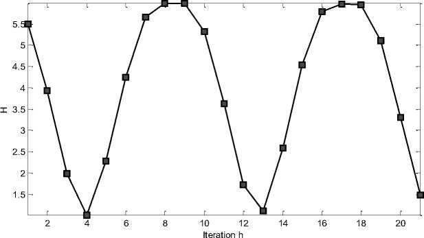
Figure 4. Shannon entropy simulation of Grover’s QSA dynamics with five inputs
Fig. 4 shows that for five inputs of the Grover’s QSA an optimal number of iterations, according to minimum of the Shannon entropy criteria for successful result, is exactly four. With more iterations the probability of obtaining a correct answer will decrease and the algorithm may fail to produce a correct answer.
The theoretical estimation for 5 inputs gives n 42 = 4.44 iterations. The Shannon entropy-based termination condition provides the number of iterations. More detailed description of the information-based termination condition is presented below.
Simulation results of a fast Grover QSA are summarized in Table 3.
The number of iterations for the fast algorithm is estimated according to the termination condition based on minimum of Shannon entropy of the quantum intelligent state vector.
The following approaches were used in the simulations listed in Table 3.
In Approach 1, the quantum operators are applied as matrices, elements of quantum operator matrices are calculated dynamically according to Eqs. (6), (12), (4.30) and (31).
As shown in Fig. 5, the classical hardware limit of this approach to simulation on a desktop computer is around 20 or more qubits, caused by an exponential temporal complexity.
Table 3. Temporal complexity of Grover’s QSA simulation on 1.2 GHz computer with two CPUs
|
n |
Number of iterations h |
Temporal complexity , seconds |
|
|
Approach 1 (one iteration) |
Approach 2 ( h iterations) |
||
|
10 |
25 |
0.28 |
~0 |
|
12 |
50 |
44 |
~0 |
|
14 |
100 |
99.42 |
~0 |
|
15 |
142 |
489.05 |
~0 |
|
16 |
201 |
2060.63 |
~0 |
|
20 |
804 |
- |
~0 |
|
30 |
2375 |
- |
0.016 |
|
40 |
853.549 |
- |
4.263 |
|
50 |
26.353.589 |
- |
12.425 |
Memory allocated for state vector, MB
0 5 10 15 20 25
Qubit number
Figure 5. Spatial complexity of Grover QA simulation
In Approach 2, the quantum operators are replaced with classical gates. Product operations are removed from the simulation as described above. The state vector of probability amplitudes is stored in compressed form (only different probability amplitudes are allocated in memory).
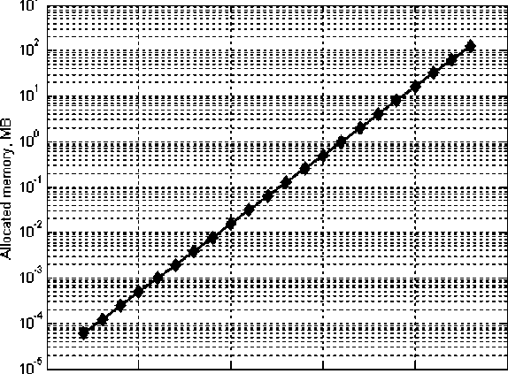
Fig. 6 shows that with the second approach, it is possible to perform classical efficient simulation of Grover’s QSA on a desktop computer with a relatively large number of inputs (50 qubits or more).
Fig. 6 shows also that with allocation of the state vector in computer memory, this approach permits simulation 26 qubits on a conventional PC with 1GB of RAM. By contrast, Fig. 5 shows memory required for Grover’s algorithm simulation when the entire state vector is stored in memory. Adding one qubit doubles the computer memory needed for simulation of Grover's QSA when state vector is allocated completely in memory.
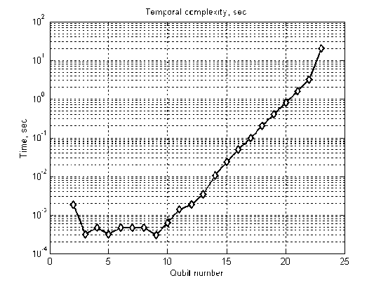
Figure 6. Temporal complexity of Grover's QSA
5. Information criteria for solution of the QSA-termination problem
Quantum algorithms come in two general classes: algorithms that rely on a Fourier transform, and algorithms that rely on amplitude amplification. Typically, the algorithms include a sequence of trials. After each trial, a measurement of the system produces a desired state with some probability determined by the amplitudes of the superposition created by the trial. Trials continue until the measurement gives a solution, so that the number of trials and hence, the running time are random.
The number of iterations needed, and the nature of the termination problem (i.e., determining when to stop the iterations) depends in art on the information dynamics of the algorithm. An examination of the dynamics of Grover’s QSA algorithm starts by preparing all m qubits of the quantum computer in the state | s ) = 10.. .0}. An elementary rotation in the direction of the sought state | x0 } with property f ( x 0) = 1 is achieved by the gate sequence:
Q = -
( ih ® 2 m ) • iXo • h
- ®2 m
k times where the phase inversion I with respect to the initial state s is defined by
4 5 = -| 5^, /J5) = 5 (x ^ 5). The controlled phase inversion I with respect to the sought state |x0) is defined in an analogous way. Because the state x is not known explicitly but only implicitly through the property f (x0 ) = 1, this transformation is performed with the help of the quantum oracle. This task can be achieved by preparing the ancillary of the quantum oracle in the state |a0} = —7= (| 0) - Ц) as the unitary and V 2
Hermitian transformation: UF : | x , a^ ^ | x , f ( x ) Ф a^ .
Thus, x is an arbitrary element of the computational basis and a is the state of an additional ancillary qubit. As a consequence, one obtains the required properties for the phase inversion I , namely:
I x, f ( x ) Ф a 0 ^ = | x ,0 Ф a0^
1 n
[| x ,° -| x ,1) ] = | x, a 0) ,
for x ^ x0
I x, f ( x ) Ф a 0 ^ = | x ,1Ф a^
[I x ,1) —| x ,° ]=— x , a йу
for x = x 0.
In order to rotate the initial state s into the state x one can perform a sequence of n such rotations and a final Hadamard transformation at the end, i.e., Ssfm = h HQ n\ sin ). The optimal number n of repetitions of the gate Q in Eq. (33) is approximately given by
----n— - 1 ~ n 72 m ,(2 m >>1).
< _ m A 2 4 '
4arcsin 2 2
V 7
The matrix D , which is called the diffusion matrix of order n , is responsible for interference in this algorithm. It plays the same role as QFT n (Quantum Fourier Transform) in Shor’s algorithm and of nH in Deutsch-Jozsa’s and Simon’s algorithms. This matrix is defined as
[ D. L, =
( - 1)1 AND (i = j ) 2 n /2
where i = 0,...,2 n - 1, j = 0,...,2 n - 1 n is a number of inputs.
The gate equation of Grover’s QSA circuit is the following:
G Grover = [( d n 0 i) . и f ] h , ( n+1 H) . (36)
The diagonal matrix elements in Grover’s QSA-operators (as shown, for example, in Eq. (37) below) are connected to a database state to itself and the off-diagonal matrix elements are connected to a database state and to its neighbors in the database. The diagonal elements of the diffusion matrix have the opposite sign from the off-diagonal elements.
The magnitudes of the off-diagonal elements are roughly equal, so it is possible to write the action of the matrix on the initial state (see Table 4).
Table 4. Diffusion matrix definition
|
Dn |
|0..0> |
|0..1> |
|i> |
|1..0> |
ll..l> |
||
|
|0..0> |
■i+ia*-1 |
l№-i |
l№-i |
Ш^1 |
l№-i |
||
|
O..l> |
1/2пЛ |
-l+lti^-1 |
1№-! |
l/2n-1 |
1№-! |
||
|
|i> |
1/2"-1 |
l№-i |
Л+Ш*-1 |
1/2"-! |
l№-i |
||
|
|1..0> |
1/2пЛ |
1/2M |
№-1 |
-1+1/211-1 |
1/2M |
||
|
lll> |
Ш*-1 |
1№-1 |
l№-i |
1/2"-! |
-l+l^^1 |
For example:
|
^- a b b b b b a |
( 1 A |
- a + ( N - 3 ) b |
|||
|
b - a b b b b |
1 |
- a + ( N - 3 ) b |
|||
|
b b - a b b b |
- 1 |
1 |
+ a + ( N - 1 ) b |
1 |
|
|
b b b - abb |
1 |
Nn " |
- a + ( N - 3 ) b |
V N |
|
|
b b b b - a b |
1 |
- a + ( N - 3 ) b |
|||
|
V b b b b b - a 7 |
V 1 7 |
v- a + ( N - 3 ) b 7 |
where a = 1 - b, b = -^y . If one of the states is marked, i.e., has its phase reversed with respect to that of the others, the multimode interference conditions are appropriate for constructive interference to the marked state, and destructive interference to the other states. That is, the population in the marked bit is amplified. The form of this matrix is identical to that obtained through the inversion about the average procedure in Grover’s QSA. This operator produces a contrast in the probability density of the final states of the database
1 2 1 2
of —[a + (N -1)b J for the marked bit versus — [a -(N - 3) b J for the unmarked bits; where N is the number of bits in the data register.
Grover’s algorithm gate in Eq. (36) is optimal and it is, thus, an efficient search algorithm. Thus, software based on the Grover algorithm can be used for search routines in a large database. Grover’s QSA includes a number of trials that are repeated until a solution is found. Each trial has a predetermined number of iterations, which determines the probability of finding a solution. A quantitative measure of success in the database search problem is the reduction of the information entropy of the system following the search algorithm.
Entropy Ssh ( p ) in this example of a single marked state is defined as
N
S ( P ) = - Z P log P , i = 1
where P is the probability that the marked bit resides in orbital i .
In general, the Von Neumann entropy is not a good measure for the usefulness of Grover’s algorithm. For practically every value of entropy, there exist states that are good initializes and states that are not. For example, S ( p( „ 4) _ mix ) = kg N - 1 = S ( p _L_j- pure j , but when initialized in p( n - 1 ) - mix , the Grover algorithm is not good at guessing the market state.
Another example may be given using pure states H00H and H1 1H. With the first, Grover finds the marked state with quadratic speed-up. The second is practically unchanged by the algorithm.
The information intelligent measure 5r (| T ) of the state | T with respect to the qubits in T and to the basis B = {| i )®---® i )} is
3 r (I T ) = 1 -
S T- (| T ) - S V (| T )
T
The intelligence of the QA state is maximal if the gap between the Shannon and the von Neumann entropy in Eq. (39) for the chosen resultant qubit is minimal. Information QA-intelligent measure 37(| T ) and interrelations between information measures S S (| T ) > S VN (| T ) are used together with entropic relations of the step-by-step natural majorization principle for solution of the QA-termination problem.
From Eq. (39) it can be seen that for pure states max 3r(| T) i—> 1 - min
Г s (IT)-ST (IT)
min S ^ (| T ) , S T N fl T ) = 0 . (40)
From Eq. (39) the principle of Shannon entropy minimum is described as follows.
According to Eq. (40), the Shannon entropy shows the lower bound of quantum complexity of the QA. It means that the criterion in Eq. (40) includes both metrics for design of an intelligent QSA: (i) minimal quantum query complexity; and (ii) optimal termination of the QSA with a successful search solution.
The Shannon information entropy is used for optimization of the termination problem of Grover’s QSA. A physical interpretation of the information criterion begins with an information analysis of Grover’s QSA based on using of Eq. (4.39). Thus Eq (4.39) gives a lower bound on the amount of entanglement needed for a successful search and of the computational time.
A QSA that uses the quantum oracle calls { O 5} as I - 2| s ^l calls the oracle at least
T >
r 1 - P v 2n
1 ^
n log N v
N
times to achieve a probability of error P . The information system includes the
N — state data register. Physically, when the data register is loaded, the information is encoded as the phase of each orbital. The orbital amplitudes carry no information. While state-selective measurement gives as result only amplitudes, the information is hidden from view, and therefore, the entropy of the system is maximum: S S^ ( p ) = — log ( 1/ N ) = log N .
The rules of quantum measurement ensure that only one state will be detected each time.
If the algorithm works perfectly, the marked state orbital is revealed with unit efficiency, and the entropy drops to zero. Otherwise, unmarked orbitals may occasionally be detected by mistake. The entropy reduction can be calculated from the probability distribution, using Eq. (38). The minimum Shannon entropy criteria is used for successful termination of Grover’s QSA and realized in this case in digital circuit implementation.
Fig. 7 shows the results of entropy analysis for Grover’s QSA according to Eq. (32), for the case where n = 7, f ( X o ) = 1.
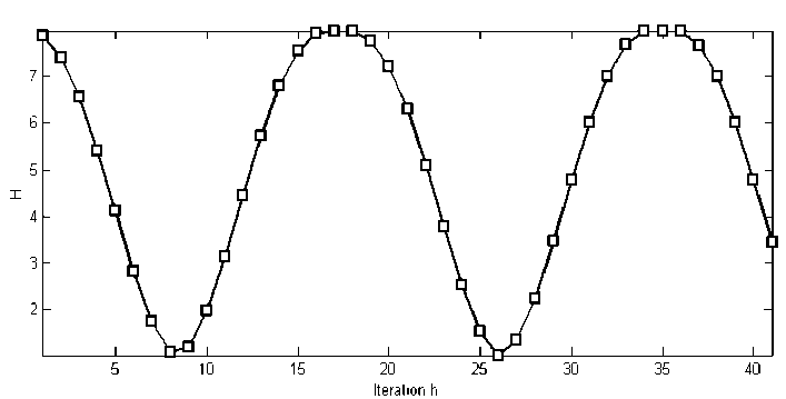
Figure 7. Shannon entropy simulation of QSA with 7- inputs
Fig. 7 shows that minimum Shannon entropy is achieved on the 8th iteration (the minimum value of the Shannon entropy is 1). A theoretical estimation for this case is n427 « 9 iterations. On the ninth iteration, the probability of the correct answer already becomes smaller, and as a result, measurement of the wrong basis vector may happen.
Application of the Shannon entropy termination condition is presented below for different input qubit numbers of Grover’s QSA. For efficient termination of QAs that give the highest probability of successful result, the Shannon entropy is minimal for the step m + 1. This is the principle of minimum Shannon entropy for termination of a QA with the successful result. This result also follows from the principle of QA maximum intelligent state. For this case:
max JTr (| ^ ) = 1
—
. HT (I ^ )
min
T
S VN (| ^ ) = 0 (for pure quantum state).
Thus, the principle of maximal intelligence of QAs includes as particular case the principle of minimum Shannon entropy for QA-termination problem solution.
6. Structure and acceleration method of quantum algorithm simulation
The analysis of the quantum operator matrices that was carried out in the previous sections forms the basis for specifying the structural patterns giving the background for the algorithmic approach to QA modeling on classical computers. The allocation in the computer memory of only a fixed set of tabulated (pre-defined) constant values instead of allocation of huge matrices (even in sparse form) provides computational efficiency. Various elements of the quantum operator matrix can be obtained by application of an appropriate algorithm based on the structural patterns and particular properties of the equations that define the matrix elements. Each representation algorithm uses a set of table values for calculating the matrix elements. The calculation of the tables of the predefined values can be done as part of the algorithm’s initialization.
-
6.1. Algorithmic representation of the Grover’s QA
Figs 8 (a--c) are flowcharts showing realization of such an approach for simulation of superposition (Fig. 8 (a)), entanglement (Fig. 8 (b)) and interference (Fig. 8 (c)) operators in Grover’s QSA.
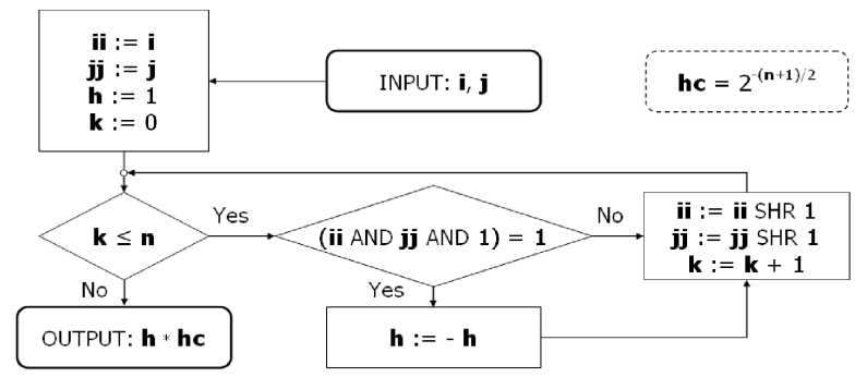
Figure 8 (a). Superposition operator representation algorithm for Grover’s QSA
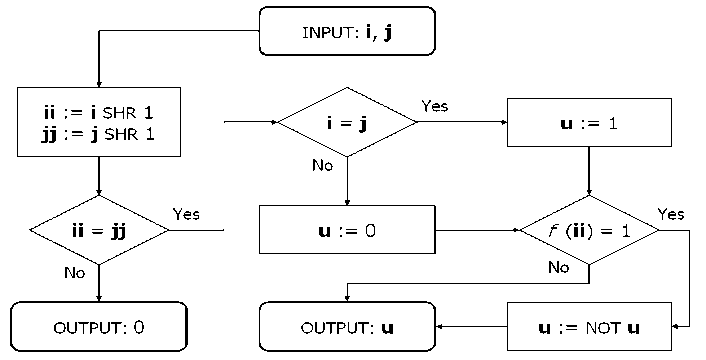
Figure 8 (b). Entanglement operator representation algorithm for Grover’s QSA
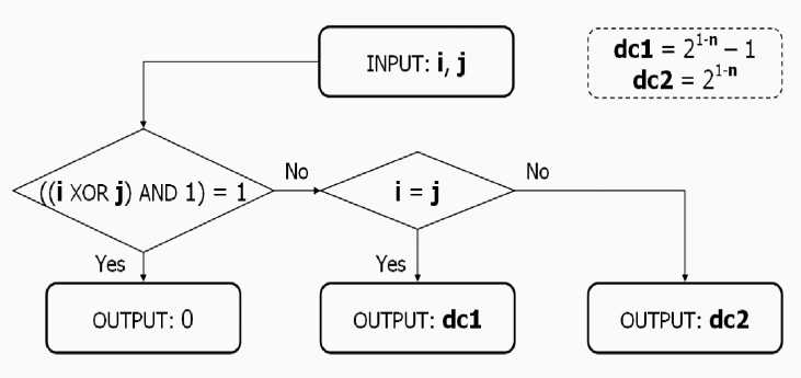
Figure 8 (c). Interference operator representation algorithm for Grover’s QSA
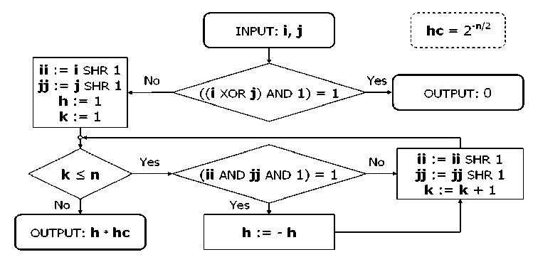
Figure 8 (d). Interference operator representation algorithm for Deutsch-Jozsa’s QA
Here n is a number of qubit, i and j are the indexes of a requested element, hc =2-(n+1)/2, dc 1 = 21-n – 1 and dc 2 = 21-n are the table values.
In Fig . 8 (a), the i,j values are specified and provided to an initialization block with loops control variables ii := i , jj := 0, and k := 0 are initialized, and calculation variable h := 1 is initialized. The process then proceeds to a decision block. In the decision block, if k is less than or equal to n , then the process advances to another decision block; otherwise, the process advances to an output block, where the output h*hc is computed (where hc = 2 - ( n + 1)/2). In the decision block, if ( ii and jj and 1) = 1, then the process advances to a block h : = - h ; otherwise, the process advances to another block and passes to the next iteration without probability amplitude inversion. Alternatively, the process sets h: = - h and proceeds to the next iteration. By setting ii : = ii SHR 1, jj : = jj SHR 1, and k := k + 1 (where SHR is a shift right operation), and then the process continues until all probability amplitudes are assigned.
In Fig. 8 (b), the inputs i, j in an input block are initialized as ii : = i SHR 1, and jj : = SHR 1 and then are passed to the end test.
If the end test is not succeeding, means the inputs i and j are pointing to the marked elements, the process of the probability amplitude inversion of the marked states in this case is performed.
In Fig. 8 (c), interference operator of Grover’s QSA can be substituted by a simple logic which outputs 0 if (( i XOR j ) AND 1) = 1 then regarding nonzero elements, if i = j then the process outputs dc 1, otherwise the process outputs dc 2, where dc 1 = 21- n – 1 and dc 2 = 21- n.
As described above, the superposition and entanglement operators for Deutsch-Jozsa’s QA are the same with superposition and entanglement operators for Grover’s QSA (Figs 8 (a), and 8 (b), respectively). The interference operator representation algorithm for Deutsch-Jozsa’s QA is shown in Fig. 8 (d), where hc = 2- n/2
The entanglement operator for the Simon QA is shown in Fig. 8 (e). Here m is an output dimension, ec 1 = 2 m – 1 and ec 2 = 2 m-1 are the table values.
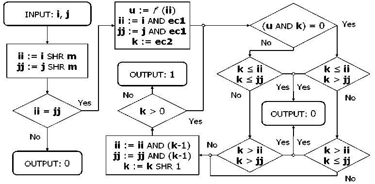
Figure 8 (e). Entanglement operator representation algorithm for Simon’s and Shor’s QA
Superposition and interference operators for the Simon QA are identical (see Table 1) and are shown by flowchart in Fig. 8 (f).
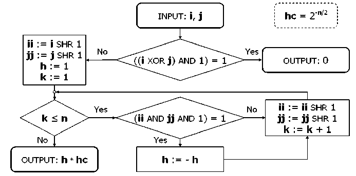
Figure 8 (f): Superposition and interference operator representation algorithm for Simon’s QA Fig. 8 (g) is a flowchart showing calculation of the interference operator from the Shor QA.
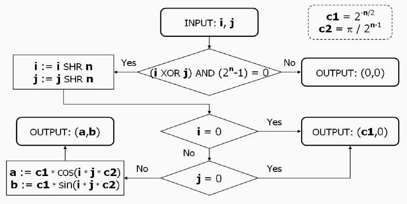
Figure 8 (g). An interference operator representation algorithm for Shor’s QA
The Shor interference operator is relatively more complex, as explained above. Superposition and entanglement operators for the Shor algorithm are the same as the Simon’s QA operators shown in Fig. 8 (f) and Fig. 8 (e). The Shor interference operator is based on the Quantum Fourier Transformation (QFT) with table values c1 = 2 – n/2 and c2 = π /2 n – 1.
The time required for calculating the elements of an operator’s matrix during a process of applying a quantum operator is generally small in comparison to the total time of performing a quantum step. Thus, the time burden created by exponentially increasing memory usage tends to be less, or at least similar to, the time burden created by computing matrix elements as needed. Moreover, since the algorithms used to compute the matrix elements tend to be based on fast bit-wise logic operations, the algorithms are amenable to hardware acceleration.
Table 5 shows comparisons of the traditional and as-needed matrix calculation when the memory used for the as-needed algorithm (Memory* denotes memory used for storing the quantum system state vector).
-
*The results shown in Table 5 are based on the results of testing the software realization of Grover QSA simulator on a personal computer with Intel Pentium III 1 GHz processor and 512 Mbytes of memory. Only one iteration of the Grover QSA was performed.
-
6.2. Problem-oriented approach based on structural pattern of QA state vector
Table 5 shows that significant speed-up is achieved by using the algorithmic approach as compared with the prior art direct matrix approach. The use of algorithms for providing the matrix elements allows considerable optimization of the software, including the ability to optimize at the machine instructions level. However, as the number of qubits increases, there is an exponential increase in temporal complexity, which manifests itself as an increase in time required for matrix product calculations.
Table 5. Different approaches comparison: Standard (matrix based) and algorithmic based approach
|
Qubits |
Standard |
Calculated Matrices |
||
|
Memory , MB |
Time , s |
Memory * |
Time , s |
|
|
1 |
1 |
0.03 |
≈ 0 |
≈ 0 |
|
8 |
18 |
4 |
0.008 |
0.0325 |
|
11 |
1048 |
1411 |
0.064 |
2.3 |
|
16 |
-- |
-- |
2 |
4573 |
|
24 |
-- |
-- |
512 |
3*108 |
|
64 |
-- |
-- |
-- |
-- |
Use of the structural patterns in the quantum system state vector and use of a problem-oriented approach for each particular algorithm can be used to offset this increase in temporal complexity. By way of explanation, and not by way of limitation, the Grover algorithm is used below to explain the problem-oriented approach to simulating a QA on a classical computer.
Let n be the input number of qubits. In the Grover algorithm, half of all 2 n + 1 elements of a vector making up its even components always take values symmetrical to appropriate odd components and, therefore, need not be computed.
Odd 2 n elements can be classified into two categories:
-
- The set of m elements corresponding to truth points of input function (or oracle); and
-
- The remaining 2 n - m elements.
The values of elements of the same category are always equal.
As discussed above, the Grover QA only requires two variables for storing values of the elements. Its limitation in this sense depends only on a computer representation of the floating-point numbers used for the state vector probability amplitudes. For a double-precision software realization of the state vector representation algorithm, the upper reachable limit of q-bit number is approximately 1024.
Fig. 9 shows a state vector representation algorithm for the Grover QA.
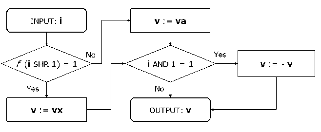
Figure 9. State vector representation algorithm for Grover’ quantum search
In Fig. 9, i is an element index, f is an input function, vx and va corresponds to the elements’ category, and v is a temporal variable. The number of variables used for representing the state variable is constant. A constant number of variables for state vector representation allow reconsideration of the traditional schema of quantum search simulation.
Classical gates are used not for the simulation of appropriate quantum operators with strict one-to-one correspondence but for the simulation of a quantum step that changes the system state. Matrix product operations are replaced by arithmetic operations with a fixed number of parameters irrespective of qubit number.
Fig. 10 shows a generalized schema for efficient simulation of the Grover QA built upon three blocks, a superposition block H , a quantum step block UD and a termination block T .
Fig. 10 also shows an input block and an output block. The UD block includes a U block and a D block. The input state from the input block is provided to the superposition block. A superposition of states from the superposition block is provided to the U block. An output from the U block is provided to the D block. An output from the D block is provided to the termination block. If the termination block terminates the iterations, then the state is passed to the output block; otherwise, the state vector is returned to the U block for iteration.

Figure 10. Generalized schema of simulation for Grover’ QSA
As shown in Fig. 11, the superposition block H for Grover QSA simulation changes the system state to the state obtained traditionally by using n + 1 times the tensor product of Walsh-Hadamard transformations. In the process shown in Fig. 10, vx:= hc, va:= hc , and vi:= 0 , where hc = 2 - (n+1) / 2 is a table value.
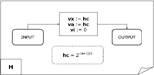
Figure 11. Superposition block for Grover’s QSA
The quantum step block UD that emulates the entanglement and interference operators is shown on Figs 12 (a – c).
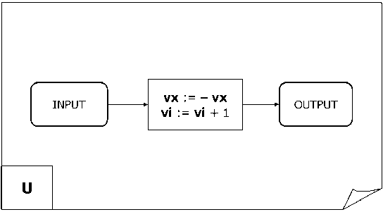
Figure 12 (a). Emulation of the entanglement operator application of Grover’s QSA
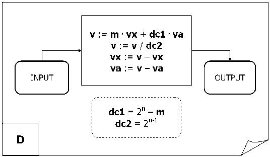
Figure 12 (b). Emulation of interference operator application of Grover’s QSA
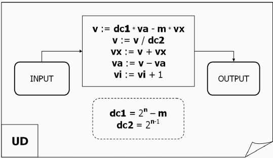
Figure 12 (c). Quantum step block for Grover’ quantum search
The UD block reduces the temporal complexity of the quantum algorithm simulation to linear dependence on the number of executed iterations. The UD block uses recalculated table values dc 1 = 2 n - m and dc 2 = 2 n-1.
In the U block shown in Fig. 12 (a), vx := - vx and vi := vi + 1.
In the D block shown in Fig. 12 (b), v := m * vx + dc 1* va , v := v / dc 2, vx := v - vx , and va:= v - va in the UD block shown in Fig. 12 (c), v:= dc1*va = m*vx , v:=v/dc 2, vx := v + vx, va := v - va , and vi := vi + 1.
The termination block T is general for all QAs, independently of the operator matrix realization. Block T provides intelligent termination condition for the search process. Thus, the block T controls the number of iterations through the block UD by providing enough iteration to achieve a high probability of arriving at a correct answer to the search problem. The block T uses a rule based on observing the changing of the vector element values according to two classification categories. The T block during a number of iterations, watches for values of elements of the same category monotonically increase or decrease while values of elements of another category changed monotonically in reverse direction. If after some number of iteration the direction is changed, it means that an extremum point corresponding to a state with maximum or minimum uncertainty is passed. The process can using direct values of amplitudes instead of considering Shannon entropy value, thus, significantly reducing the required number of calculations for determining the minimum uncertainty state that guarantees the high probability of a correct answer.
The termination algorithm realized in the block T can be used one or more of five different termination models:
Model 1: Stop after a predefined number of iterations;
Model 2: Stop on the first local entropy minimum;
Model 3: Stop on the lowest entropy within a predefined number of iterations;
Model 4: Stop on a predefined level of acceptable entropy; and/or
Model 5: Stop on the acceptable level or lowest reachable entropy within the predefined number of iterations.
Note that models 1 — 3 do not require the calculation of an entropy value.
Figs 13 — 15 show the structure of the termination condition blocks T .
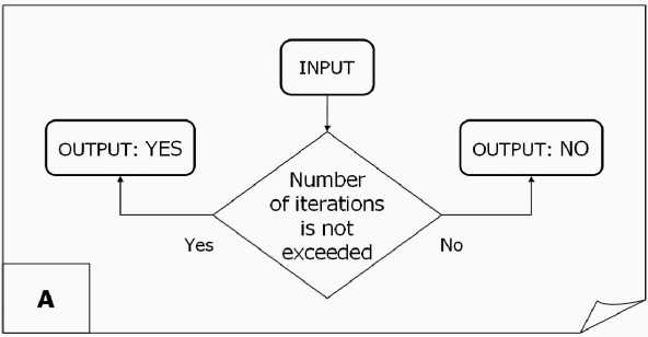
Figure 13. Termination block for method 1
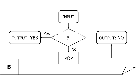
Figure 14. Component B for the termination block
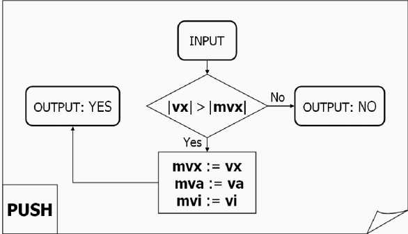
Figure 15 (a): Component PUSH for the termination block
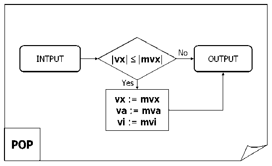
Figure 15 (b). Component POP for the termination block
Since time efficiency is one of the major demands on such termination condition algorithm, each part of the termination algorithm is represented by a separate module, and before the termination algorithm starts, links are built between the modules in correspondence to the selected termination model by initializing the appropriate functions’ calls.
Table 6 shows components for the termination condition block T for the various models. Flow charts of the termination condition building blocks are provided in Figs 13 – 15.
Table 6. Termination block construction
|
Model |
T |
B’ |
C’ |
|
1 |
A |
-- |
-- |
|
2 |
B |
PUSH |
-- |
|
3 |
C |
A |
B |
|
4 |
D |
-- |
-- |
|
5 |
C |
A |
E |
The entries A, B, PUSH , C, D, E , and PUSH in Table 6 correspond to the flowcharts in Figs 13 — 18 respectively.
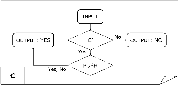
Figure 16. Component C for the termination block
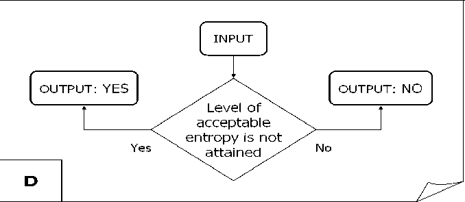
Figure 17. Component D for the termination block
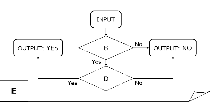
Figure 18. Component E for the termination block
In model 1, only one test after each application of quantum step block UD is needed. This test is performed by block A . So, the initialization includes assuming A to be T , i.e., function calls to T are addressed to block A . Block A is shown in Fig. 13.
As shown in Fig. 13, the A block checks to see if the maximum number of iterations has been reached, if so, then the simulation is terminated, otherwise, the simulation continues.
In model 2, the simulation is stopped when the direction of modification of categories’ values are changed. Model 2 uses the comparison of the current value of vx category with value mvx that represents this category value obtained in previous iteration:
-
(i) If vx is greater than mvx , its value is stored in mvx , the vi value is stored in mvi , and the termination block proceeding to the next quantum step;
-
(ii) If vx is less than mvx , it means that the vx maximum is passed and the process needs to set the current (final) value of vx := mvx , vi := mvi , and stop the iteration process. So, the process stores the maximum of vx in mvx and the appropriate iteration number vi in mvi . Here block B , shown in Fig. 14 is used as the main block of the termination process.
The block PUSH, shown in the Fig. 15 (a) is used for performing the comparison and for storing the vx value in mvx ( case a ). A POP block, shown in Fig. 15 (b) is used for restoring the mvx value ( case b ). In the PUSH block of Fig. 15 (a), if | vx | > | mvx |, then mvx := vx , mva := va , mvi := vi , and the block returns true; otherwise, the block returns false.
In the POP block of Fig. 15 (b), if |vx| <= |mvx|, then vx:= mvx, va:= mva , and vi := mvi .
The model 3 termination block checks to see that a predefined number of iterations do not exceed (using block A in Fig. 13):
-
- If the check is successful, then the termination block compares the current value of vx with mvx . If mvx is less than, it sets the value of mvx equal to vx and the value of mvi equal to vi . If mvx is less using the PUSH block, then perform the next quantum step;
-
- If the check operation fails, then (if needed) the final value of vx equal to mvx , vi equal to mvi (using the POP block) and the iterations are stopped.
-
- The model 4, the termination block uses a single component block D , shown in Fig. 17.
The D block compares the current Shannon entropy value with a predefined acceptable level. If the current Shannon entropy is less than the acceptable level, then the iteration process is stopped; otherwise, the iterations continue.
The model 5 termination block uses the A block to check that a predefined number of iterations do not exceeded. If the maximum number is exceeded, then the iterations are stopped. Otherwise, the D block is then used to compare the current value of the Shannon entropy with the predefined acceptable level. If acceptable level is not attained, then the PUSH block is called and the iterations continue. If the last iteration was performed, the POP block is called to restore the vx category maximum and appropriate vi number and the iterations are ended.
Fig. 19 shows measurement of the final amplitudes in the output state to determine the success or failure of the search.
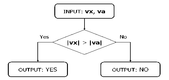
Figure 19. Final measurement emulation
If | vx | > | va |, then the search was successful; otherwise, the search was not successful.
Table 7 lists results of testing the optimized version of Grover QSA simulator on personal computer with Pentium 4 processor at 2GHz.
Table 7. High probability answers for Grover QSA
|
Qbits |
Iterations |
Time |
|
32 |
51471 |
0.007 |
|
36 |
205887 |
0.018 |
|
40 |
823549 |
0.077 |
|
44 |
3294198 |
0.367 |
|
48 |
13176794 |
1.385 |
|
52 |
52707178 |
267 |
|
56 |
210828712 |
20.308 |
|
60 |
843314834 |
81.529 |
|
64 |
3373259064 |
328.274 |
The theoretical boundary of this approach is not the number of qubits, but the representation of the floating-point numbers. The practical bound is limited by the front side bus frequency of the personal computer. Using the above algorithm, a simulation of a 1000 qubit Grover QSA requires only 96 seconds for 108 iterations (see below).
The above approach can be used for simulation of the Deutsch-Jozsa’s QA. The general schema of Deutsch-Jozsa’s QA simulation is shown on Fig. 20, where an input state is provided to a quantum HUD block, which generates an output state.
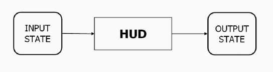
Figure 20. Generalized schema of simulation for Deutsch-Jozsa’s QA
The structure of the HUD block is shown in Fig. 21, where the input is provided to an initialization block.
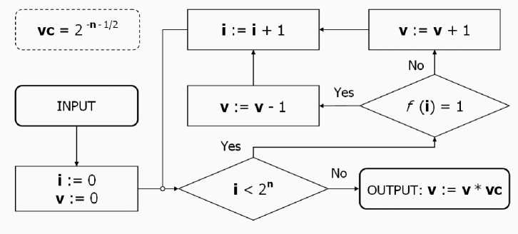
Figure 21. Quantum block HUD for Deutsch-Jozsa’s QA
The initialization block sets i := 0 and v := 0, and then the process advances to a decision block. In the decision block, if i < 2n, then the process advances to a decision block 3; otherwise, the process advances to an output block which outputs v:= v*vc , where vc = 2 - n - 1/2 .
The quantum block HUD is applied only once to obtaining of the final state. Here v represents the vector |0…00> amplitude, f is an input function of order n , vc = 2 - n - 1/2 is a table value.
After applying the block HUD, the value of v is considered in correspondence with Table 8.
Table 8. Possible answers for Deutsch-Jozsa’s problem
|
Value of v |
Answer |
|
0 |
f is balanced |
|
1 V 2 |
f is constant 0 |
|
1 — ----- - 2 |
f is constant 1 |
|
Otherwise |
f is something else |
References Algorithmic representation of the quantum operators and fast quantum algorithms
- Ulyanov S.V., Litvintseva L.V., Ulyanov I.S. et all. Quantum information and quantum computational intelligence: Classically efficient simulation of fast quantum algorithms (SW&HW implementations). - Note del Polo Ricerca. - Milano: Universita degli Studi di Milano Publ, 2004. - Vol. 79. - URL: http://www.qcoptimizer.com.
- Ulyanov S.V. Efficient simulation system of quantum algorithms on classical computer based on fast algorithm: Patent US 2006/0224547 A1. - 2006.
- Ulyanov S.V. Fast algorithm for efficient simulation of quantum algorithm gates on classical computer // Systemics, Cybernetics and Informatics. - 2004. - Vol. 2. - № 3. - Pp. 63-68.
