Algorithmic Tricks for Reducing the Complexity of FDWT/IDWT Basic Operations Implementation

Recently, a discrete wavelet transform (DWT) has been used in numerous computer graphics, signal and image processing applications [1-11].

In 1989, Stéphane Mallat proposed a fast wavelet decomposition and reconstruction algorithm [1]. The basic idea of the fast algorithm is, in case of both 1D DWT and 2D DWT, the decomposition of the original signal (or image) using a pair of filters (high- and low-pass) on two components and following the decomposition of the low pass component in the same hierarchical manner. This decomposition process is called analysis. The inverse process is called reconstruction (or synthesis) [3, 5, 7].

The cores of multilevel DWT decomposition and reconstruction procedures are forward DWT (FDWT) and inverse DWT (IDWT) “basic operations” – the multiplication of data vector by FDWT or IDWT base matrix, which describes the filter coefficients [12].

In the matrix-vector form FDWT basic operation can be defined in the following way:

• (l)                  (l)

Y2x1 = F2xLXLx1 , l 0,1,k..., Nl 2    1

While the inverse operation used to recreate signal from DWT coefficients (inverse DWT base operation) looks as demonstrated in (2):

X^ =(F2x JT Y2(l)

L X1       2X L2

where N – is a number of the original signal samples, L – is a size of sliding window that defines the part of the signal processed by the given base operation, k = 0,1,...K — 1 - is a decomposition step number indicating the granularity degree of data resolution, K – the total number of the decomposition steps.

Vector Y(l) = [y2и y^+1]T - is a two-element output data vector for each basic operation (1)-(2), where y and y     are, respectively, detail and approximation components, which are computing as a result of the execution of FDWT basic operations.

Vector X⁽_L' ^ = [ x_2I , x _2Z+1 ,..., x _z+2Z-1 ] ^T in (1) represents a column vector of length L whose elements represent the corresponding sequence of signal samples and vector X L X 1 = [~ 2 1 ,~ 2 1 + 1 ,...,~ L + 2 1 — 1 ] ^{T in (2)} represents ^the approximation of the vector X ^{( l )} obtained as a result of the reconstruction of initial data from two-element vector DWT coefficients Y ^{( l )} .

F 2 x L =

Matrix c 0      C1      c 2    Л  cL-1

. cL -1   - cL-1   cL -3   Л   - c0 _ in (1) is a FDWT base matrix with dimensions of (2 x L), whose elements represent the coefficients of the high-pass and low-pass filter respectively. Formulas (1), (2) define FDWT and IDWT basic operation respectively [12].

From expressions (1) and (2) it is clear that the implementation of the FDWT basic operations required to perform 2 L multiplications and 2( L - 1) additions whereas the implementation of the IDWT basic operations required to perform 2 L multiplications and L additions. In this paper some algorithmic tricks that reduce the number of multiplications in the implementation of the FDWT/IDWT basic operations are demonstrated.

Minimizing the number of multiplications is especially important in the design of specialized VLSI mathematical or DSP processors because reducing the number of multipliers also reduces the power dissipation and lowers the cost implementation of the entire system being implemented. Moreover, a hardware multiplier is more complicated unit than an adder and occupies much more chip area than the adder. Even if the chip already contains embedded multipliers, their number is always limited. This means that if the implemented algorithm has a large number of multiplications, the projected processor may not always fit into the chip and the problem of minimizing the number of multiplications remains relevant.

In this paper two approaches to the synthesis of rationalized algorithms for implementation of FDWT/IDWT basic operations are considered. In the first approach, the reduction of the number of multipliers in the implementation of the FDWT/IDWT basic operations is achieved by applying the Winograd’s inner product formula. Another approach uses effective schemes of matrix factorization described in [13]. It should also be noted that during the construction of algorithms the extensive use of the principles of parallelization and vectorization of data processing will be made. Therefore, it is assumed that the synthesized procedures will be implemented on the hardware platforms with parallel processing.

• II.    R ationalized A lgorithms F or F dwt /I dwt B asic O perations I nplementation U sing W inograd ’S I nner P roduct F ormula

• A.    Background

Let ^X N x 1 = ^[ x 0 , xV—x N - 1 ] ^and Y M x 1 = ^[ y 0 , y 1 >'"> y M - 1^{] -}be N -point and M -point one dimensional data vectors respectively, and m = 0, M - 1, n = 0, N - 1.

The calculation of product poses a problem

V = A X

Y M x 1   A M x N X N x 1 .

According to Winograd’s formula for the inner product calculation each element of vector Y can be calculated as follows [14]:

ym

N - 1

= E ^[( a m ,2 k + ^X 2 k + 1⁾⁽ a m ,2 k + 1 + ^X 2 k ^{)] -} 5 m ^- ^ ^M ) k = 0

Where

5 m

N - 1

'm ,2 k "  a m ,2 k + 1 and ^ ^{( M} ) = E x 2 k "  x 2 k + 1 k = 0

N - 1 E a. k = 0

if N is even.

It should be emphasized that if matrix A    is a constant coefficient matrix, ^ can be calculated in advance. The calculation of £(M) requires the N/2 multiplications to be performed. By exploiting some rationalization solutions based on application of the Winograd’s inner product formula, the number of multipliers, necessary for fully-parallel implementation multipliers could be decreased.

• B.    Rationalized algorithm for FDWT basic operation implementation using Winograd’s inner product formula

In the beginning, when using the elements of the matrix F , a column vector will be formed:

^^               ^^

F3 Lx1 = [CL x1,0 L x1,C L X1]T where

(2Лх, = [c0,c,...,cL_,]T - is a column vector containing the impulse response coefficients of the low pass filter, c^lx 1 = [Cl-1,-Cl-2,...-Co]T - is a column vector containing the impulse response coefficients of the high pass filter, and 0   - is a column vector or matrix of size defined by low subscript and consisting of all zeros.

Next, we introduce some auxiliary matrices:

- matrix of data duplication  P3ixL = 13x3® IL , where 13x1 = [1, 1,1]T here and further in this paper, is a matrix of size defined by a low subscript and consisting of all 1s, ® - is a

Kronecker product sign [15];

- permutation matrix P_3i = I_3l ® J₂

where

I - here and further in this article, is an identity matrix of size defined by low subscript, J - is an exchange matrix of size defined by low subscript, where the 1 elements reside on the counter diagonal and all other elements are zero;

- partial products summation matrix

A з l = I 3 ® 1 l 3x—         1x—

and

^F 24 _x 1     ^{[ C} 0 , ^C1 ,,." ^C 7 ,⁰,⁰,--'⁰, ^c 7 , ^c 6 ,""" - ^C 0 ^] .

Whereas the computational procedure for this example takes the following form:

^Y 2 x 1 = ⁰ 2 x 1 ^{+ K} 2 x 3 ^A 3 x 12 ^{[ R} 12 x 24 ^{O ( P} 24 ^F 24 x 1 ^{+ P} 24 x 8 ^X 8 x 1 )   (4)

- vector 6 2 x 1 = [ +^В -S,^{] T} , В = ^ c 2 i • c 2i _{+ 1} ;

i = 0

where в = c ₀ C 1 + c ₂ c ₃ + c ₄ c 5 + c ₆ c 7 ,

- matrices

	"1	- 1	0"
R 3 L     1 3 L 0 1 1 x 2 and K 2 x 3 —x3 L   — 22	. 0	- 1	1

Taking into account the introduced vector-matrix constructions, the FDWT basic operation computational procedure with a reduced number of multiplications (or multipliers in case of hardware implementation) can be represented as follows:

Y2x1 =02x1+KA зl [R3lо

3x——x3

о(Рз L F3 L x1 + P3 LxL X L x1)](3)

The operator “ о ” named “vectorized Hadamard product” [12, 13] has been introduced for the convenience of the description of the simultaneous selected vector elements multiplication procedure – it will transform certain data column vector X into the output column vector Y in a following way:

YM x1 = BMxN о X N x1 , where BMxN =| К, n|| , m = 0, M - 1, П = 0, N - 1 — is a binary mask-matrix, and the elements y are determined by the following rule [12, 13]:

^P 24 x 8 = 1 3 x 1 ® I 8

У = 1

N - 1 ^ ^bm , n x n , . n = 0

N - 1

П ^bm , " x " ,

_ n = 0

N - 1

for ^ ^bm , n = ¹

N-0        v i = 0, m -1, for X bm „ > 1 m,n n=0

Let us consider a concrete example. Suppose L = 8 .

Then

F

^F 2 x 8

c ₀

c ₁     c ₂

c ₇

^{- C} 6

c ₅

c ₃

^{- C} 4

c ₄

c ₃

c ₅

^{- C} 2

c ₆

c ₁

c ₇

^{- C} 0

P ₂₄ = ( I ₄ ® J ₂ ) © 0 8 © ( I ₄ ® J ₂ ) =

	"J 2__	0 2	0 2	0 2	0 8
	0 2	J 2	0 2	0 2
	0 2	0 2	J 2	0 2
	0 2	0 2	0 2	J 2
=		0	8		0 8
	.	0	8		0 8

0 8
J 2	0 2	0 2	02
0 2	J 2	0 2	0 2
0 2	0 2	J 2	0 2

J 2 J

R 12 x 24 = I 3 ®

A A 3 x 12

0 1 x 2

⁰ 1 x 2

0 1 X 2

0 1 x 2

0 1 x 2

0 1 x 2

⁰ 1 x 2

⁰ 1 x 2

⁰ 1 x 2

0 1 x 2

0 ;;;

0 1 x 2

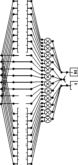
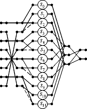
Fig. 1 shows a data flow diagram, which describes the rationalized algorithm for the implementation of FDWT basic operation for case L = 8 . In this paper, the data flow diagrams are oriented from left to right. The squares here and further in this paper denote additions with constant values inscribed in the field. The circles in all figures show the operation of the multiplication of two variables or multiplication by a constant inscribed inside a circle. Straight lines in the figures denote the operations of data transfer. Points where lines converge denote summation. The dashed lines indicate the subtraction operation. We deliberately use the usual lines without arrows on purpose, so as not to clutter the picture.

C. Rationalized algorithm for IDWT basic operation implementation using Winograd’s inner product formula

For the synthesis of rationalized calculation procedure for IDWT basic operation implementation the following matrix constructions are introduced:

- partial products summation matrix

ALx2L = (11x2 ® IL2) ® (11x2 ® IL2) , where 11X2 = [1 , -1] and ® - is direct sum sign [15],

- first permutation matrix

^P 2( L + 1) x 2 = 1 ( L + 1) x 1 ® I 2 ’

- second permutation matrix

P₃      = I, ® 1

- L x ( L + 1)     -

L x 1

® I£

2 ^,

- third permutation matrix

2 L x ³ L

= 1 2 x 1 ® I L

- fourth permutation matrix

P_2£ = I_£ ® J _L ® I_£

- column vector

C 2( L + 1) x 1 = [( I L ® J 2 ) ® 0 2 ® ( I L ® J 2 )} ® 2( L + 1) x 1

where

^Ф 2( L + 1) x 1 = [ c 0 , c L - 1 ,-", c L , c L ,⁰,⁰, c L , c L , ™ , c L - 1 , c 0 ^]

2 -      2        2   2 -

- column vector

Where

Ψ

3 L

---x1

= 0 L ■ Y L ■ 0 Lx x1 ■     x1 ■     x1

^Y L     ^[( c 0 c L - 1 )’ ⁽ c 1 c L - 2 )’

—x1

( CL_C L )] ^T 2    2

x ₀ х ₁ х ₂ х ₃ х ₄ х ₅ x ₆ x ₇

c ₇

c ₅

c ₄

c ₆

с ₂

с ₀

с ₁

c ₃

—

—

— с1

c ₆

c ₅

c ₇

c ₃

c ₄

c ₀

c ₂

y ₀

+ В -»y 1

Fig 1: Data flow diagram for FDWT basic operation ralization according to the procedure (4).

When using introduced vector-matrix constructions, the IDWT basic operation computational procedure with reduced number of multiplications (or multipliers in case of hardware implementation) can be written in the following form:

~

^X L x 1 = ^A L x 2 L ^P 2 L ^P    3 _r^{^₃    + ^P 3,    _n^{[ B} ( L + 1) x 2( L + 1) ^] °

2 L x- L    3 _{L x 1}      —L 2 ( L + 1)

° ^{( C} 2( L + 1) x 1 ^{+ P} 2( L + 1) x 2 Y 2 x 1 ⁾]^{}                              (5)}

Let us consider the next example for same L = 8 .

The computational procedure (10) for this example takes the following form: ~

^X 8 x 1 = A S x 16 ^P 16 ^P 16 x 12 { ^ _{12 x 1} ^{+ P} 12 x 9 [ B 9 x 18 ^] °

°(C18x1 + P18x2Y2x1)]}(6)

where

^P 18 x 2 = 1 9 x 1 ® ¹ 2

^C 18 x 1    ^С 18 ^Ф 2( L + 1) x 1 ,

c

C 18 x 1

[ c 7, c0,---,c3,0,0, c3, c4,"-rc7],

Ф1821   [ c 0, c 7,", c3, c 4,0,0,c 4,c 3,-",c 7, c 0],

C 18 = ( 1 4 ® J 2 ) Ф O 2 ® ( 1 4 ® J 2 ) =

J 2	0 2	0 2	0 2	0 8 x 2	0 8
0 2	J 2	0 2	0 2
0 2	0 2	J 2	0 2
0 2	0 2	0 2	J 2
0 2 x 8				0 2	0 2 x 8
0 .				0 8 x 2	J 2	0 2	0 2	0 2
					0 2	J 2	0 2	0 2
					0 2	0 2	J 2	_02.
					0 2	0 2	0 2	J 2

^ 12 x 1     ^{[ 0} 4 x 1 , ^Y 4 x 1 , ⁰ 4 x 1 ^]  ,

B .   = I 9 ® 1 1 x 2 = I 9 ® [Ш] =

=	"1    1	0 1 x 2	0 1 x 2	0 1 x 2	0 4 x 2	0 4 x 8
	0 1 x 2	11	0 1 x 2	0 1 x 2
	0 1 x 2	0 1 x 2	11	0 1 x 2
	0 1 x 2	0 1 x 2	0 1 x 2	11
					11
	0 4 x 8 L				0 4 x 2	11	0 1 x 2	0 1 x 2	0 1 x 2
						0 1 x 2	11	0 1 x 2	0 1 x 2
						0 1 x 2	0 1 x 2	11	0 1 x 2
						0 1 x 2	0 1 x 2	0 1 x 2	1    1 _

Y 4 x 1 =

c ₀ c ₇

c ₁ c ₆

c ₂ c ₅

c ₃ c ₄

, ^ 12 x 1 = [ 0 4 x 1 , Y 4 x 1 , 0 4 x 1 ] ^T

0 0

c ₀ c ₇ c ₁ c ₆ c ₂ c ₅ c ₃ c ₄ 0 0 0 0

P 16 = I ₈ © J 4 © I 4

P 16 =

,

^P 16 x 12 = 1 2 x 1 ® I;

.

y ₀ y ₁

c ₇

с ₀

^— c 6

с ₁

c ₅ с ₂

— c c3

—

—

c ₃ c ₄ c ₂ c ₅ с ₁ c ₆ c ₀ c ₇

~ _{x 0} ~ _{x 1} x

^ x ₃ x ₄ ~ _{x 5} ^~ x ₆

x

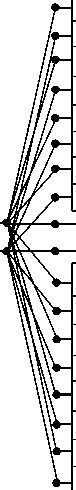
Fig 2: Data flow diagram for IDWT basic operation ralization according to the procedure (6).

III. Rationalized Algorithm For Fdwt/Idwt Basic Operations Execution Using Gauss’ Trick For 2×2 Matrix Factorization

A. Short background

Let us rearrange the columns of the matrix F so that a new matrix takes the following form:

F = F P

¹ 2x L    *-2x L¹-L

where

Р_£ = || p ,J is a permutation matrix whose elements are defined as follows:

Fig. 2 shows a data flow diagram, which describes the rationalized algorithm for the implementation of IDWT basic operation for case L = 8 .

The proposed algorithms allow the total number of multiplications to be reduced, relative to the direct method. The number of multiplications in the algorithm for the implementation of FDWT/IDWT basic operations represented by the procedure (3) is 1,5 L . On the other hand, the algorithm for the implementation of FDWT basic operation, represented by the procedure (3) requires only (3,5 L + 1) additions, instead of 2( L — 1) in the direct algorithm. The number of multiplications in the algorithm for the implementation of IDWT basic operations represented by the procedure (5) is L + 1 . In turn, the algorithm for the implementation of IDWT basic operation, represented by the procedure (5) requires 3,5 L additions.

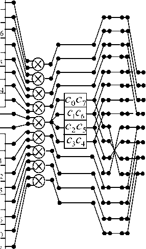
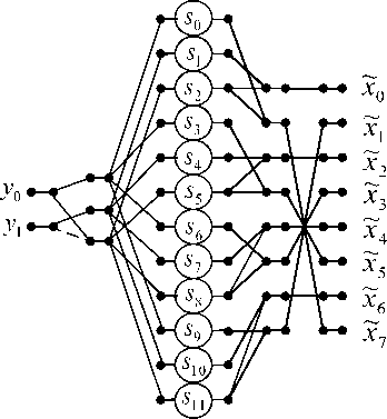
L p2i+1,2i+1 = 1, i = 0

.

The computation process for the multiplication of matrix F^~by vector X can be implemented as L/2 independent vector-matrix products with 2 x 2 matrices. The results of these calculations should be later added. We will notice that all sub blocks of the new matrix F^~ possess specific block structures. This specificity, as we show below, allows the reduction of the number of multiplications in the implementation of the partial vector-matrix products. The mentioned possibility of rationalization uses the following decomposition [13]:

a	b"		"0	1	1
c	a	=	1	0	1

c - a	0	0"	"1	0
0	b - a	0	0	1
0	0	a	_1	1

structures will have the following form:

As can be seen, each of such vector-matrix multiplications requires only three multiplications and five additions. The use of singularities can offer a more cost-effective way to obtain a set of partial vector-matrix products. Below the application of this trick is considered in detail.

• B.    Rationalized algorithm for FDWT basic operation implementation using Gauss’s matrix factorization trick

At first we extract elements from F matrix to create a new diagonal matrix:

L-i

D 3l = ® D3i), —   i=0

where submatrices

^D3¹) = diag[(h(L-1)-2i - h2i), ⁽h(L-1)-2i + h2i ), h2i^]   are ^{3 X 3}

diagonal matrix.

Next we introduce three types of summation matrices:

A 3 L = (I L ® T3 2) - matrix of pre-additions, — X L-

• A, 3L = (IL ® T_{2 3}) - matrix of post-additions,

L x —-

А 3 L = (1 t ® I3) - partial results summation matrix, 3x—1x—

A

^A 12x8

1 1 1   -1 1 1 1   -1 1 1 1  - 1 1 1 1  - d12 = e d(i), 12    i=0

D3i) = diag[(c7-2i - c2i ),(c7-2 i + c2i ), c2i ] , matrix and

T

' 2x3

1   - 1

Taking into account introduced vector-matrix constructions, the FDWT basic operation computational procedure with a reduced number of multiplications can be represented as follows:

(l)                                                              (l)

Y2x1 = ^t2x3a, 3L ^D3L A3L pLXLx1 3x— — —xL

D12 = diag (s o, s1, s 2, s 3, s 4, s 5, s 6, s 7, s 8, s 9, s_w, s_n),

s 0 c 7 c 0  ,   ^s1   c7 + c 0  ,   s 2   c 0  , s 3   c5   c 2

s 4 — c 5 + c 2 , ^s 5 — c 2 , s 6 — c3   c4 , s 7 — c 3 + c4 , s 8 — c 4 ,

s 9 = ^C1   c6, s10 = ^C1 + c6, s11 = c 6 ,

^A3x12 =

C. Rationalized algorithm for IDWT basic operation implementation using Gauss’matrix factorization trick

The basic operation computational procedure takes the following form:

We consider against an example for L = ⁸

Then

~(l)(

XLX1 = PLAT 3L D3L P3L „ T3x2 Y2x1

Lx— ——x3

(l)          (3)                                     (l)

Y2x1   ^T2x3A3x12^D12A12x8^r8^A8x1               ⁽⁸⁾

Where

Thus the previously introduced vector-matrix

A 3 L = I L ® ^T2x3 , ^P3 L  = A, 3 L^.

Lx—   —          —x3    3x —

22     2    2

For our example the matrices P8, D12 , P12x3 = A^2 , T , and T have been defined above, just as the matrix

A _3L

L x— 2

is defined as follows:

A ^л 8x12

Fig 4: Data flow diagram for IDWT basic operation ralization according to the procedure (10).

Then, for this example, the IDWT basic operation computational procedure takes the following form:

^~(l)                                           (l)

^X8x1   ^P8A8x12D12^P12x3 T3x2 Y2x1

The data flow diagrams for the execution of FDWT and IDWT basic operations in accordance with the procedures (8) and (10), are shown in Figures (3) and (4), respectively.

х₄

x х1 х2 х х5

x₆

x

y₀ y₁

Fig 3: Data flow diagram for FDWT basic operation ralization according to the procedure (8).

The number of multiplications in the algorithm for the implementation of FDWT/IDWT basic operations, represented by the procedure (7), is 1,5L . On the other hand, the algorithm for the implementation of FDWT basic operation, represented by the procedure (7), requires only (2L -1) additions, instead of 2(L -1) in the direct algorithm. The number of multiplications in the algorithm for the implementation of IDWT basic operations represented by the procedure (9), is 1,5L . In turn, the algorithm for the implementation of IDWT basic operation, represented by the procedure (9), requires L +1 additions.

• IV. Conclusion

We see that the solutions proposed in this article allow to reduce the total number of multiplications in the implementation of FDWT/IDWT basic operations compared to the naive methods of computing. Indeed, in the general case a fully parallel implementation of FDWT/IDWT basic procedures requires   2L multiplications. The number of multiplications for each of proposed here algorithms is 25% less than that of the direct execution of computations.

It is noteworthy that, because all elements in F matrix are constants, we can (but not must) use one-input units (encoders), instead of traditional multipliers. In such case, it is apparently advisable to use the second approach for the implementation of the FDWT/IDWT basic operations. This solution    greatly simplifies implementation, reduces the power dissipation and lowers the price of the device. On the other hand, when we are dealing with FPGA chips that already contain a number of embedded multipliers, the construction and usage of additional encoders instead of multipliers is irrational. In this case, it would be unreasonable to refuse the possibility of using embedded multipliers. In this case, any algorithms derived from the application of both approaches can be used with approximately equal effect.

The algorithms proposed in this article allow the number of multiplications to be reduced at the cost of more additions, or more complex memory access. Such solutions make no sense in some modern high-speed architectures, where pipelined fixed-point or floatingpoint addition and multiplication take just one clock cycle. Therefore, the solutions presented here are intended solely for the hardware implementation of FDWT/IDWT basic operations.