Amodified probabilistic genetic algorithm for the solution of complex constrained optimization problems

The necessity to develop complex system models appears in different fields of science and technology such as mathematics, economics, medicine, spacecraft control andsoon. In the process of modeling there emerge many optimization problems which are multiextremal, multiobjective and have implicit formalized functions, complex feasible area structure, many types of variables etc. There is no possibility to solve such problems using classical optimization procedures thus we have to design and implement more effective and universal methods such as genetic algorithms (GAs). GAs proved their efficiency in the process of solving of many complex optimization problems [1; 2].

The GAs efficiency depends on fine tuning and control of their parameters. If an untrained user sets arbitrary parameters values, the GA efficiency may vary from very low to very high. The recent trends in a field of GAs are adaptive GAs based on complex hybrid structures and efficient GAs with reduced parameters set.

A known approach to GA parameters set reduction is probabilistic genetic algorithms (pGAs) [3; 4]. The essential difference between pGA and standard GA is that pGA has no crossover operator and new solutions are generated according to statistical information about search space. Thus, collecting and processing such kind of information, pGAs can adapt to the problems they solve.

PGAs demonstrated their efficiency with many complex optimization problems and their further investigation and improvement are promising. There are actual problems of the pGA’s features analysis for wide-range optimization problems and parameters set reduction without efficiency loss. This article is devoted to pGAs efficiency for complex constrained optimization problems investigation.

Probabilistic genetic algorithm for non-constrained optimization problems. During its run the GA collects and processes some statistical information about search space, but the statistics is absent in an explicit form. PGA uses the following form of statistics representation – the probabilities vector of the current population:

р^к =( p k ,..., p k ), p k = p ( x k =1), i =1 n , here p _i ^k is the probability of unit value for i- th bit in solution X^k , k is iteration number.

The general scheme of pGA is:

• 1.    Random generation of the initial population.

• 2.    Selection of r individuals (called parents) on the basis of their fitness. Evalu at e the probabilities vector as:

• 3.    Form a new population (called offspring) according to the distribution P .

• 4.    Apply mutation operator to the offspring.

• 5.    Form a new population from parents and offspring.

• 6.    Repeat 2–5 steps.

^P = (А,-, P n ) ,

1 ^r

P j =^P { x j = 1} = E j j =1 n , r i =1

here n is chromosome length, x ⁱ _j is j -th gene of i th individual.

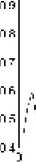
As it was previously mentioned, during pGA run the algorithm collects the statistics about null and unit values distribution in the population. The experimental results show that the probability vector components converge to the corresponding values of the optimal solution vector as shown in figure 1.

:з -j о sc зс ?! si о и

Fig. 1. The values change for j -th component of the probability vector

As it is shown in figure 1, the given j -th component value of P converges to unit. It means that the value of j -th gene of optimal solution most probably is equal to unit (for binary representation). One can use this feature to predict the optimal solution.

The following prediction algorithm was proposed in [3; 4]:

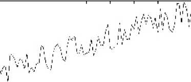
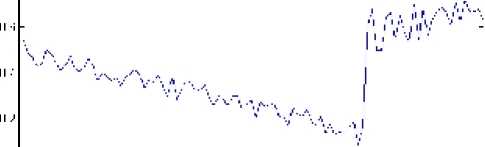
In practical problems there may be such situations when pGA collects not enough information at the beginning and j -th gene value is equal to unit (or zero) for almost every solution. At the final stage pGA can find a much better solution with inverted values of j -th gene and it means that the probability vector values will change their convergence direction (fig. 2). But the above mentioned prediction algorithm will give us the primary value, because the j -th value of probability vector was greater than 0.5 (or less than 0.5 for zero values) for a long time.

Thus one can use the following prediction algorithm modification:

• 1.    Set the prediction step K .

• 2.    Every K iteration use the given statistics P i , i = 1, N_K , N_K = t ■ K , t e { 1,2, K } to evaluate the probability vector change: A P i = P i - P i —1 .

• 3.    Set the weights for every iteration according to its number: c i = 2 i,N K^ N K +1 ) , i = 1, K , N_K .

• 4.    Evaluate the probability vector weighted change as: N K

• 5.    Set the optimal solution: X ^P = f x °^pt ), where x °^pt = 1 if A p j > 0, and x °^pt = 0 otherwise.

• 6.    Add the optimal solution in the current population and continue pGA run.

AP = (A P_j) = E°i'AP i .

i =1                            ____

и 11---------------------------------------------1----------------------------------------------1----------------------1---------------------------------------------1----------------------1----------------------------------------------

"j             Я JJ 'L 61 U .-I Я U. 111.

Fig. 2. The situation when prediction can be wrong

The main idea of the given algorithm is that the probability values on the later iterations have the greater weights as the algorithm collects more information about search space. The NK weights have values such that oi+1 > gi и E°i = 1.

i =1

Genetic algorithms for constrained optimization problems. In general GAs and pGAs select an individual in accordance with its fitness value, but there is no optimization constrains control. There are many possible methods to solve this problem.

Let the following constrained optimization problem be solved:

f ( x ) ^ extr,

^ g j ^{( x} ) ^ 0, ^j = 1, r , h j ( x ) = 0, j = r +1, m .

In general, the individual x fitness is evaluated as:

m fitness( x) = f (x) + 5 ■ X( t) ■ E fjP (x), j=1

where t is iteration number; 5 = 1 for the minimization problem; 5 = -1 for the maximization problem; f j ( x ) is the penalty value for j -th constrain break; в is the real number.

The penalty functions f_j ( x )areevaluatedas:

fj ( ^x ) = •

max { 0, gj( x ) } ,J' = 1, r | J x )|, J = r +1, m

The following penalty methods are known: the “death” penalty, the static penalty, the dynamic penalty, the adaptive penalty and hybrid methods of the individuals “cure”.

As the authors analyzed every penalty method, the further investigation was limited by the dynamic and adaptive penalty methods as other methods have a number of disadvantages.

In particular, the “death” penalty eliminates every unfeasible solution even if it can have the important information for new feasible solutions. The static penalty contains a large set of parameters that should be well tuned – a non-optimal set of parameters can lead to unfeasible solutions. The “cure” method involves local optimization procedures on every iteration of GA, thus such methods use much more computational recourses.

The dynamic penalty . The method uses the previously mentioned penalty functions and defines X( t ) in a following way:

X( t ) = ( C ■ t ) ^a .

The fitness of x individual on the t -th iteration is evaluated as:

fitness( x ) = f ( x ) + 5 ■ ( C ■ t Y^f , ^p ( x ).

i =1

The values C , а, в are set according to a certain problem. The recommended values are C = 0.5, а = р = 2 (obtained experimentally).

The adaptive penalty uses the same penalty functions, but X( t ) is evaluated as:

i p1 ■!(t), ifb € D, for t - k +1 < i < t

X( t +1) = <

в₂ ■!( t ), ifb 4 D , for t - k +1 <  i <  t ,

X(t), otherwise, where b is the best solution in the i-th population, в e (0,1), P2 > 1 and P1P2 ^ 1. The penalty decreases on the (t + 1) step, if the best individual was feasible during the last k iterations. Otherwise, if it was unfeasible, the penalty increases.

The method uses three parameters: P₁, P₂, k . The adaptive penalty method uses both kinds of information: if the solution is unfeasible and if the previous solutions was unfeasible [5].

Probabilistic genetic algorithms for constrained optimization problems. The general scheme of pGA is the same as for the penalty method. The main difference is in the fitness function definition. Thus, one can extend the optimal solution prediction method for the constrained optimization problems. It is appropriate to use the modified prediction procedure as the objective function surface with penalty can have a lot of local optima and the general prediction algorithms can lead to a local solution instead of a global one.

GA and pGA computational efficiency investigation for constrained optimization problems. We compare the algorithms efficiency on a set of test problems of single objective constrained optimization. The objective functions and constrains are linear and non-linear functions of several variables. A part of test problems set is presented in table 1 [6].

We investigate “the best-efficiency” and “the worstefficiency” parameters set for both algorithms to determine how parameters influence the efficiency in a wide range. The better results for “the worst-efficiency” parameters set give us better effectiveness for arbitrary parameters chosen by an untrained user.

AsGA and pGA are stochastic procedures, we average characteristics of algorithms with every unique parameter set over 100 independent runs.

To estimate algorithms efficiency we will use the following criteria:

• –    the rate of runs (%), where the exact optimal solution was computed;

• –    the average iteration number ( N ), on which the exact optimal solution was computed for the first time.

At the first stage we define the constrains control method that gives the best efficiency with the given test problems set. We have resumed that the standard GA with “the bestefficiency” parameters shows the best results with the dynamic penalty for the whole test problems set. The standard GA with “he worst-efficiency” parameters shows the best results with the dynamic penalty only for 60 % cases (problems). On the average, the dynamic penalty is more effective than the adaptive penalty in 60 % cases.

PGA both with “the worst-efficiency” and “the bestefficiency” parameters shows the best results with the dynamic penalty for the whole test problems set.

Thus, we have determined that the dynamic penalty is more effective than the adaptive penalty for both GA and pGA algorithms.

At the second stage we compare the efficiency of standard GA and pGA with dynamic penalty. For “the best-efficiency” parameters set the standard GA is more effective than pGA in 67 % cases. But in cases when pGA yelds to GA, their efficiency differs insignificantly. For “the worst-efficiency” and “average-efficiency” pGA is more effective than GA in 100 % and 67 % cases respectively. The computational results of comparison are given in table 2.

At the third stage we compare the efficiency of standard GA and pGA with dynamic penalty. For “the best-efficiency” parameters set the standard GA is more effective than pGA in 67 % cases. But in cases pGA yelds to GA, their efficiency differs insignificantly. For “the worst-efficiency” and “average-efficiency” pGA is more effective than GA in 100 % and 67 % cases respectively. The computational results of comparison are given in table 2.

At the forth stage we compare the efficiency of standard GA and pGA with optimal solution prediction. For «the best-efficiency» parameters set the pGA with optimal solution prediction is more effective than the standard GA in 60 % cases, “the worst-efficiency” pGA is more effective in 67 % cases. Moreover, the pGA with optimal solution prediction finds the optimal solution at much earlier iteration. The comparison of computational results are in table 3.

The results of the investigation shows that the pGA algorithm is more preferable than the standard GA, because it is more effective on the average and it has smaller number of parameters. The pGA with optimal solution prediction allows to compute optimal solution at much earlier iterations.