An adaptive image in painting method based on the modified Mumford-Shah model and multiscale parameter estimation

Image inpainting problem is one of the important problems of image processing and has wide range of application in practice. The image inpainting [1, 2, 3] is synonym for parts interpolation of image. Because of some reasons such as dusts, noises, scratches etc., many parts of old photos/films are missed and damaged. The goal of image inpainting is to restore those corrupted parts. The image inpainting can be also used for removing unnecessary objects on images, such as text erasing (watermark removal), remove special effects on image, disocclusion [4], image zooming, image super-resolution, predict objects position etc.

In recent years, the approaches to the image inpainting problem based on partial differential equations (PDEs) and calculus of variation are widely studied [1]. They still exist parallelly with other learning-based approaches due to their own advantages. In this work, we just focus on non-learning-based approaches.

In image processing, the widely recognized result is known as Shannon’s sampling theorem [5]: if an analog with finite energy does not contain any high frequencies, then it can be perfectly interpolated from its properly sampled discrete sequence as Nyquist frequency. In image inpainting, the input images are corrupted by many factors. So, to formulate the image inpainting problem by Shannon’s theorem, we need to deal with a class of unreliable sample. By variational approach, we need to find the regularity of an image that fits the ideal image well. The regularity relates to energy functionals that are formulated on, such as the Sobolev norm E [ u ] = J _q | V u | ² (known as the Tikhonov regularization) [6], the total variation

E[u] =[ IV u| [7, 8] and the Mumford-Shah image n model E[u] = J I V u |2 + aH1 (Г), where Q - the image domain, Г – the edge set, H1 – the 1D Hausdorff measure [9], a>0. Hence, by Shannon’s theorem, the image inpainting model by variational approach can be formulated as a constrained optimization problem. The Mumford-Shah model [1, 2] is a popular and effective mathematical tool to solve the image segmentation problem and other image restoration problems.

Based on the Mumford-Shah image model, Esedoglu et al. developed the modified Mumford-Shah inpainting model and its adaptive inpainting model named the Mumford-Shah-Euler inpainting model [3]. By using the Am-brosio-Tortorelli approximation method [10, 11], Ese-doglu et al. approximated the edge collection Г of the Mumford-Shah inpainting model to acquire the modified Mumford-Shah model. This method is more effective for the image inpainting problem, than the segmentation and the denoising tasks, because details of objects of the resulted image get natural and less smooth than for the segmentation and the denoising tasks. However, this model is multiparameter and it is very complex to estimate all parameters. Although we can fix two parameters of the Ambrosio-Tortorelli method, there are still two other parameters need to be estimated. The goal of this work focuses on parameters estimation of the modified Mumford-Shah inpainting model.

The estimation technique that we used in this work is the multiscale parameter estimation based on the inverse gradient [12]. The definition “multiscale” relates to solving the engineering problems that have many important features at multiple scales of time and/or space. The multiscale parameter estimation is an effective method that is widely used in many tasks of image processing and computer vision problems.

To assess the image quality after inpainting of the proposed method, we will handle experiments and compare to other similar inpainting methods: the modified Mumford-Shah inpainting model [3], the harmonic inpainting method [13, 14] (PDE-based) and the total variation inpainting method [15] (variation-based). The harmonic inpainting is an image interpolation method that focuses on finding solution of the Laplace equation or as a minimizer of Dirichlet energy over the inpainting domain. The total variation inpainting method is developed based on the total variation image reconstruction problem [16] of Rudin et al. The implementation of the total variation inpainting method is on the Nesterov optimal first-order gradient method [15]. This method is especially effective for denoising, deblurring and inpainting.

In the experiments, we consider two popular and important applications of the inpainting: restore the missing and damaged parts of image and remove objects on image. Over the experiments, the proposed method will prove the effectiveness of combination of the modified Mumford-Shah inpainting model and the multiscale parameter estimation.

The rest of the paper is organized as follows. Section 2 presents the adaptive image inpainting method: the modified Mumford-Shah image inpainting, the proposed adaptive image inpainting method, multiscale parameter estimation and other parameters configuration. Section 3 presents experimental results and the comparison with other similar inpainting methods. Finally, Section 4 concludes.

• 2.    The adaptive image inpainting method

  • 2.1.    The modified Mumford-Shah image inpainting model

Let u original ( x ), u 0 ( x ), u ( x ) e R - be the original image (ideal sample), the corrupted image and the reconstructed image, respectively; x = ( x 1 , x 2 ,…, x p ) – pixels, p = 1,2,…. If p =2, we have 2D image that is presented in the form of the matrix of pixels and this kind of image is very popular.

Mumford and Shah [17] proposed an image inpainting model by minimizing the following energy functional:

E [ u , Г , D ] =-J ( u - u ₀) 2 d x + - J | V u| ² d x + a H ¹ ( Г ) , ² Q ²

where Q - set of all image pixels (image domain), Г - set of edge pixels, D - set of corrupted pixels, X >0, y >0, a >0, V - gradient operator, |-|- L ² norm, H ¹ - the 1D Hausdorff measure [9], which generalizes the length notion for regular curves.

By using the Ambrosio-Tortorelli approximation method [10, 11], Esedoglu and Shen proposed to apply the Г – convergence approximation to the Mumford-Shah image inpainting model. They simplified the term corresponding to the Hausdorff measurement and obtained the new image inpainting model that was well-known as the modified Mumford-Shah inpainting model [3] as below:

E [ u , z | u o , D ] = ^X J ( u ² Q

- u ₀ )2 d x + — J z ² |V u |² d x + 2 Q ' '

+ ^a J ^-V z

Q I

( 1 - z ) ² ) 4 s

d x ^ min,

where z : Q^ [0,1] - the edge signature (an approximation function of the edge set Г by the Ambrosio-Tortorelli method), s - accuracy of the Ambrosio-Tortorelli method, parameters X >0, y >0. For this minimization problem, we need to find u and z .

• 2.2.    The proposed adaptive image inpainting method

We consider that parameter y in model (1) is chosen base on the characteristics of input image u ₀ : y = y ( u 0 ). So, the model (1) can be rewritten:

E [ u , z | u 0 , D ^y/ C ² Q

(

+T^|V z

( 1 — z ) 2 )

4 s

^{y ( u} 0 ) f ₂ I     |2

-----I z ² V u d x +

2 Q 1 1

The suitable value of y will improve quality of the filled pixels for corrupted parts by smoothing sense.

To solve this problem, there are many methods. In this work, we use method based on the Euler-Lagrange partial differential equation. The Euler-Lagrange system of equations for variables u and z associates to model (2):

X(u -u0^^u)-V(z2Vu) = 0,(3)

(y( u 0 )|Vu|2) z + af-2sAz + z^-"j = 0,(4)

where A - Laplace operator.

The boundary conditions:

du=0, |z=0,(5)

dn where n – the normal.

The system of PDEs (3)–(4) with boundary conditions (5) can be solve by the finite difference schemes [16, 18].

• 2.3.    Multiscale parameters estimation

In works [12, 19], Prasath et al. proved that the inverse gradient will improve quality of the image denoising tasks. So, in this work, we choose the smooth parameter y based on the inverse gradient of the corrupted image:

y ( u 0 )

1 + kmax |Gp * Vu0|2 p where

^G p = _z exp pV 2 n

x

2 p ²

– Gaussian kernel, operator * – 2D convolution, k – constant (usually from 10^-2 to 10^- 4 ), p = 1,2,3,4,5.

With every scale p , we will get the corresponding value of | G _p * V u ₀ |. After evaluating all values of | G _p * V u ₀ | in all scales p , we will choose the maximum value | G _p * V u ₀ |². This value is used for evaluating y .

• 2.4.    Other parameters configuration

For the weight of the Ambrosio-Tortorelli term in model (2) (i.e. parameter a ) and its accuracy s , we use the default values were proposed by Ambrosio and Tor-torelli: a = 1, s = 0.005.

The data fidelity parameter X should be large enough to guarantee edge preservation and the details of objects of image are not blurred. However, if this value is too large, the convergence speed is too slow and unstable. For MATLAB and other numerical computing systems, too large value of X can cause some problems of memory. So, we use the same value was proposed in works based on the Mumford-Shah model X = 10 9 . If X is greater than this value, the difference of image quality after inpainting is a tiny bit and may be skipped. In the experiment, we will explain more detail on this value for X .

Algorithm of the adaptive inpainting method based on the modified Mumford-Shah inpainting model and multiscale parameter estimation is presented below:

ALGORITHM 1. THE ADAPTIVE IMAGE INPAINTING METHOD

Input : The corrupted image u ₀ .

Output : The reconstructed image u .

Step 1. Initialize a = 1, s = 0.005, X =10 9 .

Step 2. Estimate у by multiscale estimation:

|G p *Vu 0|² .

y( u 0 ) =

1 + k max p

Step 3. Solve system of PDEs (3), (4), (5) by the finite difference schemes method.

• 3.    Experimental results and discussions

  We handle the experiments of the adaptive image inpainting method and multiscale parameter estimation on MATLAB 2018a. The configuration of the computing system is Windows 10 Pro with Intel Core i5, 1.6GHz, 4GB 2295 MHz DDR3 RAM memory. Values of parameters by default a = 1, s = 0.005, X = 10 9 . These values are fair to compare to other similar inpainting methods based on the Mumford-Shah model, the total variation and PDEs. We compare the proposed method to the harmonic inpainting method (harmonic), the modified Mumford-Shah inpainting method (Mumford-Shah) and the total variation inpainting method (TV) with implementation based on the Nesterov optimization method.

• 3.1.    Parameter values and error metrics

There are two main parameters that affect the final inpainting quality, namely the iteration parameter i of the corresponding Euler-Lagrange PDEs, and k >0 which occurs in the inverse gradient terms of multiscale estimation. For the multiscale choice we chose the maximum of the parameter p = 5 (i.e. p = 1,2,3,4,5) and k =102, and the final terminal iteration is kept as a tolerance Tol = 10 – 14 value between two successive images in L2 norm, ||u[i+1] – u[i]] < Tol, where i – index of iteration. These values are fair to compare to the inpainting result of the modified Mumford-Shah method and the harmonic method. Otherwise, we also limit the maximum number of iterations – 20. This setting is helpful if the convergence is too slow. However, in all of our tests, the loop has not reach this condition. That means the convergence speed is very fast.

To evaluate the image quality after inpainting, we utilize the following error metrics [6, 7, 8, 20]:

PSNR = 10log₁₀ I -max- I dB , ( MSE )

where mn

|SE(u(,)- uoг)2 mse = Хе_±1__—---- (mn)

is the means square error with u original is the original (latent) image, m × n – size of image, u max denotes the maximum value, e.g. for 8-bit images u max = 255; u ^{( ij )} and u _o ^{( i} _r ^j _i ⁾ _ginal are the intensity of inpainted image and original image at pixel ( i , j ), respectively. Note that a difference of 0.5 dB is visible and higher PSNR (measured in decibels – dB) indicate better quality image. Structural similarity (SSIM) is a proven to be a better error metric for comparing the image quality and it is in the range [0, 1] with value closer to one indicating better structure preservation. The SSIM is computed between two windows to 1 and to ₂ of common size m x n ,

(2Ц-Ц- + c )(2^ - + c2 )

SSIM = "7--------------—,--------------7 ,

( ц ^ +Ц 2.2 ^{+ c} 1 )l> 2. ■ ⁿ to . ⁺ c 2 )

where ц_т i - the average of to i , o to , - the variance of to i , G_m 1 _m 2 - the covariance, and c 1 , c ₂ - stabilization parameters. The mean value of SSIM (MSSIM) is taken as the single value of quality indicating the structural similarity of the two images compared.

• 3.2.    Standard test images and test cases

To perform the image inpainting algorithm, we consider the following cases:

• (a)    The image inpainting was used to fill the missing and damaged parts (by dusts, scratches, noises etc.). In this case, we will evaluate the image inpainting quality and compare to other similar methods. The original images are taken from the open dataset of UC Berkeley https://www2.eecs.berkeley.edu/Research/Projects/CS/vis ion/bsds/BSDS300/html/dataset/images.html . We will generate the masks for the tests.

• (b)    The second application of image inpainting that we need to test is to remove unnecessary objects on images. The input images are also taken from the open dataset of the UC Berkeley. In this case, we do not evaluate

error metric and do not compare to other methods, because there is no metric to assess the quality of objects removal. We just focus on vision and feeling. Hence, the comparison in this case is not objective.

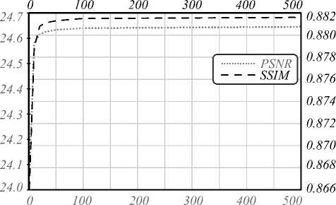
Fig. 1. Dependence of the image quality metrics (PSNR, SSIM) on parameter λ

Figure 1 shows the dependence of the image quality metrics (PSNR, SSIM) on parameter λ . This test is for the eagle image (ID 42049) with mask 3, but the result is similar with other images with various masks. We can see that, with λ > 100, the image quality by PSNR and SSIM changes very little. So, the image quality of inpainting will not depend on parameter λ anymore, if we fix the value λ = 10⁹ for all tests. Then, the difference of PSNR/SSIM values is only at the sixth digit of precision. In our experiments, we only take up to 4 digits of precision and there is no difference for PSNR and SSIM values from the point λ = 10⁶ and higher. By this way, we reduced the number of parameters of the modified Mumford-Shah model from 4 down to 2. Two other parameters were set by default based on the Ambrosio-Tortorelli approximation. Hence, in all experiments, we fixed the value λ = 10⁹, because with higher value of λ , the image quality after inpainting are quite same.

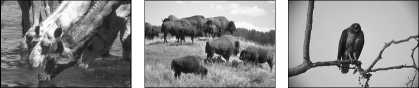
1607           38092          42049

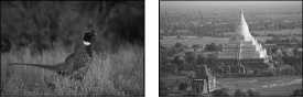
43074          76053

182053         157055         163085

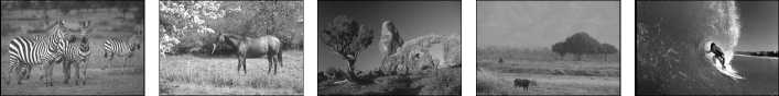
253027         291000         295087         296007         300091

Fig. 2. The input image for the proposed adaptive image inpainting method

Table 1. The inpainting results for eagle image + mask 1, plane image + mask 2, surfer image + mask 3

45 © S	-о © о и	'S © к	■я 5 -в Е -=5 S	> н	-о
й ш ь	22.4446	36.0101	36.7151	36.6754	36.7297
	14.4101	36.9052	36.3819	35.9552	37.4926
	4.3624	25.5773	24.9596	24.9937	25.6870
S ш ш	0.9118	0.9904	0.9904	0.9893	0.9929
	0.7580	0.9880	0.9800	0.9862	0.9901
	0.0379	0.7603	0.6940	0.7568	0.7709

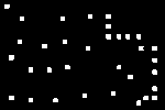
Mask 1

Mask 2

Fig. 3. The masked images

Mask 3

Figure 2 shows the selected images of the dataset of UC Berkeley. The file name (or ID) is under every image.

All images are stored in JPEG format, grayscale and size – 481×321 pixels. These images are published to use as free license.

For the first case, we use three masked images of Figure 3. The white color parts are the corrupted parts on original images that need to be recovered. We also need to notice that, all input images and the masked images are stored in the JPEG format and they are compressed (with unknown compression ratio). So, the edges around the masked on corrupted images are slightly different to the original masks. However, we can also consider that the different parts are also corrupted parts of the original images that we need to recover.

Figures 4–6 present the inpainting results by the harmonic method, the modified Mumford-Shah method, the TV inpainting method and the proposed method. Figure 4 – inpainting result for the eagle image with the mask 1, figure 5 – for the plane image with the mask 2, figure 6 – for the surfer image with the mask 3. The results of inpainting quality by the PSNR and SSIM metrics are showed in Table 1. The first row of PSNR and first row of SSIM are for the eagle image, the second ones – for the plane image, the third ones – for the surfer image.

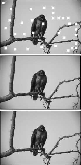
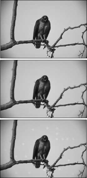
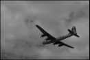
Fig. 4. Inpainting results with mask 1 for the eagle image (ID 42049): a) Original image, b) Corrupted image, c) Harmonic, d) Mumford-Shah, e) TV, f) Proposed method

This is watermain

a)

c)

e)

b)

f)

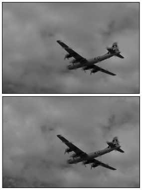
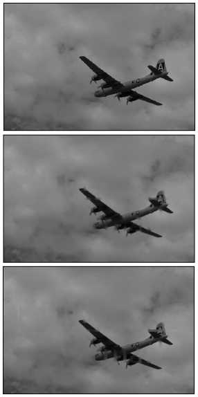
Fig. 5. Inpainting result with mask 2 for the plane image (ID 3096): a) Original image, b) Corrupted image, c) Harmonic, d) Mumford-Shah, e) TV, f) Proposed method

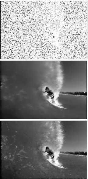
The inpainting result for the eagle image and the plane image are slightly different if we assess by human eyes. For the surfer image, our proposed method preserves the detail of the wave, the water surface and the man. Inpainting by modified Mumford-Shah is blur and lost objects details. The harmonic inpainting method and the TV inpainting are slightly better, but the detail of face and hands in TV inpainting case are lost. Inpainting result by our proposed method is slightly better than the harmonic inpainting, but it is difficult to see that difference. The Table 1 shows the image quality by PSNR/SSIM of the inpainting. By these metrics, our proposed method won in three test cases in both PSNR and SSIM sense.

The SSIM metric is more important than PSNR. SSIM is qualitative metric reflects the feeling of human vision, PSNR is quantitative metric. So, in the next experiment, we test on all images with mask 3 and we just focus on the SSIM metric.

The Table 2 shows the SSIM metric of the inpainting results for other images with the mask 3. In this case, all images are corrupted fully, and we cannot see objects on images (Figure 6). The error metrics by SSIM reflected its damaged level – nearly close to zero. We can also see that our proposed method is better than others in all test cases and surely for the average SSIM.

In the second case, we test our proposed method for the object removal. We use the soldiers image (ID 170057) and the plane image (ID 3096). We need to remove the group of soldiers from the top (for soldier image) and the plane from the sky (for plane image). The results are presented in Figure 7. The first column is for the soldiers image and the second one – for the plane image. The first row is original image. The second row is images with the marked objects need to be removed. The marked process is performed by human. We used the brush tool to mark objects that we need to remove. The last row is images after removing marked objects.

Table 2. The SSIM metric of the inpainting results for other images with mask 3

\    ’в ©JD \ 5 Q \ EH \	о U	"E о S SS Щ	■o о — IS	> H
42049	0.1218	0.8785	0.8802	0.8811	0.8817
3096	0.0345	0.9599	0.9510	0.9644	0.9644
300091	0.0379	0.7603	0.6940	0.7568	0.7709
16077	0.0755	0.6816	0.6462	0.6590	0.7080
38092	0.1458	0.6635	0.6410	0.6505	0.6742
43074	0.0170	0.7971	0.7065	0.7807	0.7990
76053	0.0409	0.6855	0.5753	0.6590	0.7181
103070	0.0283	0.7900	0.7027	0.7579	0.8066
119082	0.0701	0.6128	0.6357	0.6364	0.6533
126007	0.0382	0.7831	0.7228	0.7772	0.7904
157055	0.1195	0.7048	0.6753	0.6951	0.7088
163085	0.0240	0.7587	0.7009	0.7235	0.7791
170057	0.0427	0.7474	0.6508	0.7030	0.7563
182053	0.0753	0.7086	0.7102	0.6910	0.7271
219090	0.0475	0.7251	0.6954	0.7276	0.7493
220075	0.0463	0.7767	0.7514	0.7443	0.7953
253027	0.0575	0.6618	0.6053	0.6363	0.6761
291000	0.1134	0.4247	0.4363	0.4185	0.4541
295087	0.0254	0.7016	0.6438	0.6940	0.7161
296007	0.0459	0.7912	0.7033	0.7794	0.8094
SSIM	0.0604	0.7306	0.6864	0.7168	0.7469

For the plane image, the result after removing objects is very good. We cannot see any defects on the resulted image. However, for the soldiers image, the corresponding parts of removed objects on resulted image are slightly blur. This is a disadvantage of all inpainting methods. It happens when the area of removed objects is large and/or image parts around the removed objects are sharpened or they own many details.

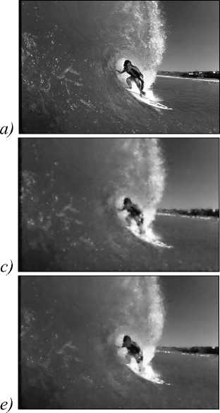
Fig. 6. Inpainting result with mask 3 for the surfer image (ID 300091): a) Original image, b) Corrupted image, c) Harmonic, d) Mumford-Shah, e) TV, f) Proposed method

b)

a)

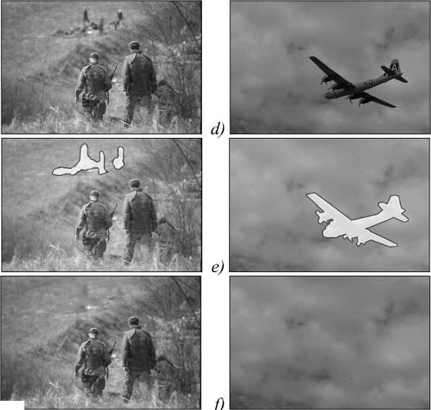
Fig. 7. The objects removal result of the proposed method

c)

Because our proposed inpainting method is an iterative manner, so the performance depends on the tolerance. With the above settings, our proposed method takes up to 11 seconds to complete the inpainting task. This is result is just slightly different to the modified Mumford-Shah inpainting method, the total variation inpainting method and the harmonic methods.

• 4.    Conclusions

In this work, we proposed an adaptive image inpainting method based on the modified Mumford-Shah model and multiscale parameter estimation. The multiscale parameter estimation was evaluated on the inverse gradient of the corrupted images to preserve the image structure.

The multiscale parameter estimation is a good method to estimate the best fitting value for γ . Otherwise, this method is also helpful to reduce the dependence of the image quality after inpainting on parameter λ . So, the proposed method reduced the number of parameters of the modified Mumford-Shah inpainting model.

The experiments also prove that our proposed method is better than the modified Mumford-Shah inpainting method, the TV inpainting method and the harmonic inpainting method by PSNR and SSIM senses. The proposed method is not only helpful for restoring old images/films that are corrupted by dusts, noises, scratches etc., but also for removing unnecessary objects on images.

One disadvantage of our proposed inpainting method and other inpainting methods is automatic detection task of the corrupted parts (mask). This task requires other learning-based techniques. In future, we will combine the deep learning to detect the complex corrupted parts on image. It is necessary to create an automatic inpainting method without any human interference.