An Algorithm for the Simulation of Pseudo Hexagonal Image Structure Using MATLAB

Published Online June 2016 in MECS DOI: 10.5815/ijigsp.2016.06.07

There exist only three possible regular tessellation schemes to cover a plane without overlapping among the samples and gaps between them [1]. They are the tessellation with squares, with hexagons, and with regular triangles. Fig.1 (a) is the square, which is familiar and usual because it is aligned with the standard Cartesian axes, which helps to make operations simple. Fig.1 (c) illustrates the triangular case, which yields a denser packing than the square case. This means that more information is contained in the same area of the image. The tessellation in Fig.1 (b) is the hexagonal case. It is believed to be the most efficient tessellation scheme among them because of its advantages like smaller quantization error Consistent Connectivity pixel is equidistantly adjacent to their six neighbours along the six sides of the pixels and Grater Angular Resolution. In addition to these advantages the primary motivation behind using a hexagonally re-sampled image is that retina of the human eye closely resembles a hexagonal grid space [2]. So we can obtain natural behaviour to realize the computer vision by using the hexagonally sampled images.

Conventional image acquisition devices acquire images with square pixels. So conversion has to be done from square image to hexagonal image before the hexagonalbased image processing. Various simulation methods have been introduced in the past years to simulate hexagonal grid on a regular rectangular grid image. Some of these simulations schemes are resampling method, pseudo hexagonal pixel ^{[3, 4]}, virtual hexagonal structure ^{[3, 5]}, mimic hexagonal structure ^{[3, 6]} and spiral architecture ^[3, 7]

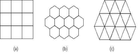
Fig.1. Three Scheme of Regular Tessellation (a) Square (b) Hexagons (c) Triangles

Two important addressing schemes used for hexagonal structure are, the row and column addressing scheme and the spiral addressing scheme.

Fig.2 shows the row and column addressing of hexagonal structure. Position of the highlighted hexagonal pixel can be considered as (3, 1), which indicate it is the element of third row and first column.

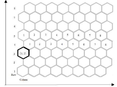
Fig.2. Row and column addressing

Sheridan [7] proposed a one dimensional addressing scheme for a hexagonal structure. This hexagonal structure is called the Spiral Architecture (SA). In the Spiral Architecture, which is shown in Fig. 3, the pixels with the shape of hexagons are arranged in a spiral clusters.

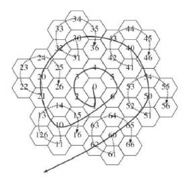
Fig.3. Spiral Architecture

In this paper an algorithm for simulating pseudo hexagonal structure using square pixel is described. Row and column addressing scheme is used in this method. The paper is organized as follows. Section 2 is literature review which includes brief description of some existing hexagonal pixel simulation methods. Section 3 is pseudo hexagonal structure simulation which describes the proposed algorithm named as ‘JK’ algorithm (where J represent the first letter of Jeevan, the first author’s name and K represent the first letter of Krishnakumar, the second author’s name). Section 4 is the discussion part and 5 is conclusion.

• II.    Literature Review

Since the cells in human retina have hexagonal structure, the image developed in the retina has hexagonal shaped pixels. In addition, hexagonal geometry has some advantage like higher sampling efficiency, consistent connectivity and higher angular resolution. Due to these reasons many researchers have studied the possibility of representing digital images with hexagonal pixels ^{[8, 9, 10, 11]}. But one difficulty we faced in hexagonal image processing is the non-availability of hardware for acquiring hexagonal images. So, rectangular grid to hexagonal grid conversion has to be done before performing hexagonal image processing. Different techniques are now available for crating hexagonal structure images. Some of these simulations schemes are re-sampling method, pseudo hexagonal pixel ^{[3, 4]}, virtual hexagonal structure ^{[3, 5]}, and mimic hexagonal structure ^[3, 6]

• A.    Resampling Method.

Re-sampling is the process of transforming a discrete image which is defined at one set of coordinate locations to a new set of coordinate points. In our case the transformation is from rectangular to hexagonal grid. Two different re-sampling methods for getting a hexagonal lattice are alternate pixel suppressal method and half-pixel shift method [12].

Hexagonal grid image based on alternate pixel suppressal method can be obtained from the conventional image by alternatively suppressing rows and columns of the existing rectangular grid and sub sampling it. All the other pixels of the rectangular grid which do not have any correspondence with the hexagonal counterparts are suppressed to zero. While processing this sub sampled image the suppressed pixels are not considered in computation [12]. The sub sampled hexagonal grid is shown in Fig. 4

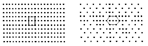
Fig.4. (a) Rectangular grid and (b) Simulated hexagonal grid obtained using alternate pixel suppression

In half- pixel shift method, for each odd line, find the midpoint between two adjacent pixels by simple linear interpolation [12]. The equation for the midpoint is shown in equation 1. Discard the left and right, keeping only the mid values. This gives us a hexagonal mapping from a regular square or rectangular grid. Fig. 5 shows the sampled grid using half-pixel shift method.

^^ _ left pixel value+rig tit pixel value         ^^

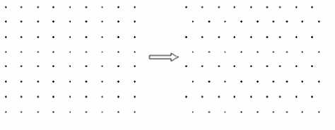
Fig.5. (a) Rectangular grid and (b) Simulated hexagonal grid using halfpixel shift method.

• B.    Pseudo Hexagonal Structure

In order to compare the visual effect of hexagonal pixel and square pixel C.A. Wuthrich and P. Stucki proposed a pseudo hexagonal pixel structure [4]. In this structure a hexagonal pixel is simulated using many square pixels. Fig. 6 shows the pseudo hexagonal pixel structure using square pixel.

• C.    Mimic Hexagona Pixels Using Square Pixel

In this method simulation one hexagonal pixel consists of four traditional square pixels and its grey level value is the average of the involved four pixels. This method preserves the important property of hexagonal architecture that, each pixel has exactly six surrounding neighbors [6].

Since the grey-level value of the mimic hexagonal pixel is taken from the average of the four corresponding square pixels, this mimic scheme introduces loss of resolution. Also the equidistance property of hexagonal representation is lost in this method. Fig.7 shows a cluster of 7 mimic hexagons.

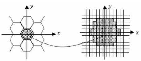
Fig.6. Pseudo hexagonal pixel.

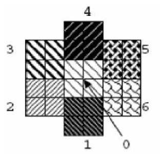
Fig.7. Cluster of 7 mimic hexagons.

• D.    Virtual Hexagonal Structure

Virtual hexagonal structure was proposed by Q. Wu, X. He and T. Hintz in their paper titled ‘Virtual Spiral Architecture’ ^{[5, 13]}. In this method, the image in conventional square grid is mapped into virtual spiral architecture. The processing is done using this virtual structure and after processing it is converted back into square grid. The block diagram in Fig.8 represents the image processing on virtual spiral architecture ^{[5, 10, 13]} .

Original Image on Square Grid

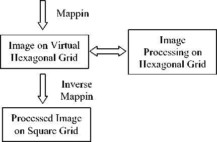
Fig.8 Image processing on virtual spiral architecture

• III.    Pseudo Hexagonal Structure Simulation

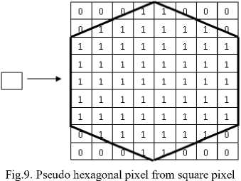
In this section an algorithm for simulating a pseudo hexagonal pixel, using square pixels is describing. The hexagonal pixel is constructed using square pixels. The procedure for constructing a hexagonal pixel using square pixels is as follows. Each square pixel is represented as a 9X8 matrix as shown in the Fig. 4. That is, 72 pixels are generated from a single pixel and the gray scale value of each pixel is same as that of the original pixel selected. Out of these 72 pixels only 56 pixels are used for making the hexagonal structure as shown in the Fig. 9. The square pixels used for creating a hexagonal pixel are labeled as ‘1’ and the remaining pixels which are labeled as 0 are discarded.

Using the above mentioned procedure, the entire square pixel in the original image can be converted to its corresponding pseudo hexagonal pixels. After converting each square pixel to its corresponding hexagonal pixels, combine all such hexagonal pixels to get the image with hexagonal structure. The Fig. 10 shows the pseudo hexagonal structure of a 3 X 3 image. The pixels are numbered from 1 to 9 as shown in the figure.

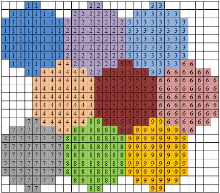
Fig.10. Hexagonal representation of a 3X3 image

Pixel numbered as 1 represents the hexagonal pixel in the first raw and first column, P(1,1). The 2nd pixel represents the pixel in the first raw and second column, P(1,2). Similarly the 9th pixel is the hexagonal pixel in the third raw and third column.

The algorithm is summarized below. The following steps are to get a single hexagonal pixel from the square pixel.

Algorithm:

{

• 1.    Read the image

• • im = imread(*.jpg)

• 2.    Get the first pixel of the image

• •    val=im(1,1);

• 3.    Define a zero matrix of size 9 X 8

• •    mat = zeros(9,8)

• 4.    Initialize two variables, row & col (column)

• •    row = 1; (for getting the desired pattern

as shown in Fig.9)

• •    col = 4; (for getting the desired pattern as shown in Fig.9)

• 5.    Assign the pixel value to the zero matrix as shown

• •    mat(row:row + 8, col:col + 1) = val;

• •    mat(row + 1:row + 7, col - 1) = val;

• •    mat(row + 1:row + 7, col + 2) = val;

• •    mat(row + 1:row + 7, col - 2) = val;

• •    mat(row + 1:row + 7, col + 3) = val;

• •    mat(row + 2:row + 6, col - 3) = val;

• •    mat(row + 2:row + 6, col + 4) = val;

• 6.    Get the pseudo hexagonal pixel

• •    Hex_Pixel = mat;

• •    Imshow(uint8(Hex_Pixel))

}

This algorithm can be extended to colour image also. The colour image includes colour information for each pixel. The colour image can be considered as the combination of three channels (or plane) namely red, green and blue planes. If the RGB image is 24-bit (the industry standard as of 2005), each channel has 8 bits, for red, green, and blue. That is, the colour image is composed of three images where each image can store discrete pixels with conventional brightness intensities between 0 and 255.

The pseudo hexagonal structure for colour image can also be obtained using JK algorithm. In the case of colour image the algorithm is performed for each channel separately. Then these three channels are superimposed to get the colour image in hexagonal structure.

• IV.    Results and Discussions

Hexagonal geometry has some advantages like higher sampling efficiency, equidistance (neighborhood pixels are at same distance), consistent connectivity (due to equidistance property), and higher angular resolution. But, the non-availability of hardware for capturing and displaying hexagonal based images limits the use of hexagonal image structure for further processing. Since there is no hardware for capturing the hexagonal images, conversion has to be done from square to hexagonal image before hexagonal-based image processing. In this work, we proposed a MATLAB based algorithm to simulate hexagonal pixels using square pixels. Since the hexagonal pixel constructed is the combination several square pixels, it is considered as pseudo hexagonal pixels. The algorithm proposed is named as ‘JK’ algorithm as mentioned in section 2.

The hexagonal structure obtained using this algorithm satisfies two important properties of hexagonal images. First one is the property of six neighbors for the central pixel. Second one is the property of consistent connectivity which is due to the same distance from the central pixel to the six neighbor pixels. These properties are illustrated in Fig. 11.

In the Fig. 11, the pixels are numbered from 0 to 6. The pixel ‘0’ is the central pixel and the other pixels are neighbors. From the figure it is clear that the central pixel is surrounded by only six neighbors. Also it is clear that the distance from the centre of the central pixel to the centre of the neighbor pixels are same. The distance to the each pixel can be calculated as follows.

From the figure, the distance from the center of the central pixel to the center of pixel 3 is measured as 8 units. The 8 units represent 8 small squares in the image. Similarly the distance to the pixel 6 is also taken as 8 units. For the other pixels (pixels 1, 2, 4 & 5), the distance can be calculated as below .

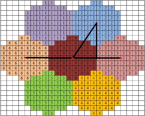
Fig.11. Six Neighbors of Hexagonal pixel.

Calculation of distance from the central pixel to pixel 2 is explained here. Same method can be used for finding the distance of pixels 1, 4 and 5 from the central pixel.

The distance from the central pixel to the starting of third pixel is measured as 4 units. Similarly the distance from the midpoint of intersection of central pixel and third pixel to the center of pixel 2 can be considered as approximately 7 units (refer Fig.11). Then using trigonometric identities we can calculate the distance from the central pixel to pixel number 2 as

√7 +4 = 8 ․ 06 ≌ 8 units          (2)

In the same manner we can calculate the distance from the central pixel to pixel 1, 4 and 5. In each case the distance found to be approximately 8 units. From the above explanation it is clear that each pixel is separated with approximately same distance.

Fig. 12 and Fig. 13 show the image with square pixel and the image with hexagonal pixel simulated using the proposed algorithm respectively.

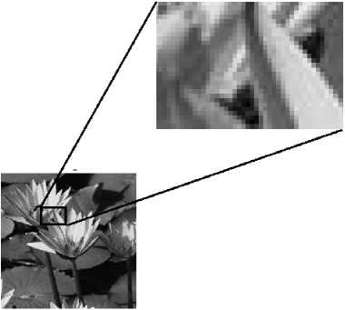
Fig.12. Original image – Image with square pixels

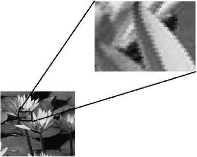
Fig.13. Image with hexagonal pixels simulated using JK algorithm

Using this algorithm we have simulated the pseudo hexagonal structure of colour image also. In the case of color image, we need to apply the algorithm for red, blue and green components separately. Fig. 14 to 16 shows some images in pseudo hexagonal structure.

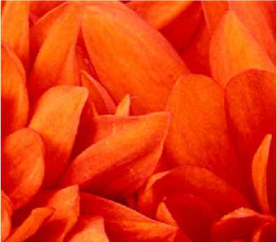
Fig.14. (a) Colour image in pseudo hexagonal structure

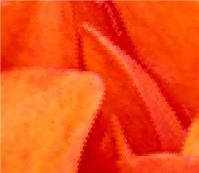
Fig.14. (b) Zoomed version of fig. 14(a)

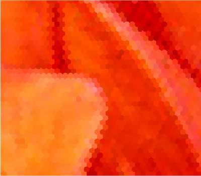
Fig.14. (c) Zoomed version (Other level) of fig. 14(a)

In the zoomed version we can identify the hexagonal shaped pixels.

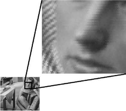
Fig.15. Image with hexagonal pixels simulated using JK algorithm

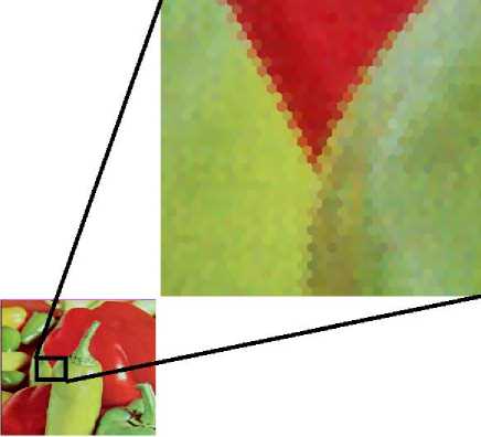
Fig.16.

• [3]    X. He, T. Hintz, Q. Wu, H. Wang and W. Jia, “A New Simulation of Spiral Architecture”, Proceeding of International Conference on Image processing, Computer Vision and Pattern Recognition, (2006) June, Las Vegas.

• [4]    C.A. Wuthrich and P. Stucki, “An algorithmic comparison between square- and hexagonal based grids”. CVGIP: Graphical Models and Image Processing, 1991. 53(4): p. 324-339.

• [5]    Q. Wu,, X. He, and T. Hintz, “Virtual Spiral Architecture”. Proceedings of the International Conference on Parallel and Distributed Processing Techniques and Applications, 2004. p. 399-405.

• [6]    X. He, “2-D Object Recognition with Spiral Architecture”, 1999, PhD Thesis, University of Technology, Sydney.

• [7]    P. Sheridan, T. Hintz, and D. Alexander, "Pseudo invariant Image Transformations on a Hexagonal Lattice," Image and Vision Computing, vol. 18, pp. 907-917, 2000.

• [8]    Middleton, L., & Jayanthi Sivaswamy, 2005, Hexagonal Image Processing– A Practical approach, USA, SpringerVerlag London Limited.

• [9]    Veni, S. & Narayanankutty, K.A., “Gabor Functions for Interpolation on Hexagonal Lattice”, International Journal of Electronics & Communication Technology, 2(1), 15-19, 2011

• [10]    Barun kumar, Pooja Gupta & KuldipPahwa, “Square Pixels to Hexagonal Pixel Structure Representation Technique”, International Journal of Signal Processing, Image Processing and Pattern Recognition, 17(4), 137-144, 2014

• [11]    Jeevan, K.M. & Krishnakumar, S. “Compression of Images Represented in Hexagonal Lattice Using Wavelet and Gabor Filter”, Proceedings of 2014 IEEE International Conference on Contemporary Computing and Informatics, pp 609 – 613, 2014

• [12]    P.Vidya, S.Veni & K.A. Narayanankutty, “Performance Analysis of Edge Detection Methods on Hexagonal Sampling Grid”, International Journal of Electronic Engineering Research, 1(4), 313-328, 2009.

• [13]    X. He, T. Hintz, Q. Wu, H. Wang and W. Jia, “A New Simulation of Spiral Architecture”, InProc.IPCV, pp 570575, 2006

• V. Conclusion

In this paper, an algorithm is proposed for simulating a pseudo hexagonal image structure using square pixels. The pseudo hexagonal structure obtained using the proposed algorithm preserve the advantages of real hexagonal structure such as uniform connectivity, equidistant property and six neighbor pixels. This method uses the row and column addressing scheme and the simulation of this structure does not require any complex computations.