An Analytical Approach to Assess and Compare the Vulnerability Risk of Operating Systems

Published Online April 2020 in MECS DOI: 10.5815/ijcnis.2020.02.01

Which operating system has served with a lower risk on so far? Are there a difference in the OS performance from the perspective of the risk associated? Answering these problems are challenging given the complexity of criteria in assessing operating systems’ performances. In the present study, authors put effort to propose a quantitative approach to assess the OSs performances. There are no specific or particular method evaluating current OSs in the market, but many different approaches from different perspectives.

Given this complexity, authors are well aware that no one comprehensive theoretical method can assess computer operating system performances, so the proposed system also have its own limitations, which will be discussed in coming sections.

However, main objective of the present study is to propose a Statistical approach based on recorded OS vulnerabilities to assess and compare performances of operating systems. Microsoft windows, Apple’s Mac and Linux are the three main PC operating systems (OS) leading in the market commanding a dominant majority of the market share. Therefore, it would not be wrong to say that in general, individual’s and organization’s information security depends largely on these three OSs efficiency. Reliability of an OS is the most important expectation for information security because OS is the mediator and the security controller of the Hardware and other application software resources of a computing system. Therefore, any Operating System is highly expected to be trusted. Achieving this reliability calls for higher quality standards in several aspects. In general a higher focus on security practices are given to detect vulnerabilities faster and then to prevent them before any exploitation occurs. This focus is mandatory and important. However, while these qualitative measures are taken, it is also important to observe the Risk associated with vulnerabilities in computer systems [2, 3].

Alhazmi, Malaiya and Ray in 2007 [2] emphasized the need for developing more quantitative approaches to address security risk related problems. Authors of the present study also support this view point since the majority of the efforts on security risk seem to have focused on qualitative approaches. Operating system security can be evaluated using many methods. A study on number of vulnerabilities discovered in an OS and their Risk level is a good index of OS security level. Ruohonen, Hyrynsalmi and Leppanen in 2015 [23] conducted an analysis on the growth of number of vulnerabilities on different operating systems and attempted a linear, logistic and Gompertz fits. There are also several scholarly attempts on forecasting the number of vulnerabilities in various aspects. Venter and Eloff in 2004 [30] proposed a conceptual model to forecast the number of vulnerabilities using several techniques with Vulnerability Scanning, Harmonized Vulnerability Category Data and Vulnerability Forecast Engine with historical data on vulnerabilities.

Assessing software product vulnerability is still an attractive and complex topic. Using historically reported vulnerabilities and number of vulnerabilities available in different vulnerability data bases is arguably the simplest method since it will calculate the total number of vulnerabilities in a software product. However, as Johnson, Gorton, Lagerstrom and Ekstedt (2016) [20] correctly pointed out, such simple numerical analysis have many limitation in assessing and understanding the vulnerability of a product. Johnson, Gorton, Lagerstrom and Ekstedt (2016) [20] therefore proposed a useful new method called “time between vulnerability disclosures (TBVD)”. The main outcome of the use of TBVD was that it would assess the software product by the effort required by an expert vulnerability analyst to find a new vulnerability in the product. This method can actually be considered as an index of a software’s susceptibility and so the reliability. Zhang, Caragea and Ou (2011) [31] suggested an approach “Time to Next Vulnerability (TTNV)”. As Johnson, Gorton, Lagerstrom and Ekstedt in 2016 [20] emphasized, this approach of TTNV also have limitations due to the fact that it rather depends on the effort and capabilities of the vulnerability analyst community in finding the vulnerability rather than the intrinsic risk in the vulnerability of the software.

Therefore it is clear that a more acceptable measure of assessing the gravity of the effects of vulnerability should mainly focus on the intrinsic risk in the vulnerability on the software system. In other words there is a need for risk measure of vulnerability based on its effect on the information security and integrity of the system. Present study therefore at first focuses on the ability to develop and use such a method that can be proposed in to the vulnerability assessment praxis of current operating systems, where the method would derive a quantitative measure for the risk of any vulnerability in an OS [24]. Second, with such a quantitative measure we shall conduct an empirical analysis on number of such vulnerabilities and then compare different OSs using the risk measure we would develop in the first step.

The article proceeds as follows. Section 2 mainly discusses Methodology with an introduction to the concept of “Risk” of a vulnerability. In addition the section will discuss the data source and currently used vulnerability scoring system. Section 3 will step by step presents the analysis and the process of assessing the risk of any vulnerability as a risk index. Both Parametric and Non Parametric [5, 8, 9, 16] outcomes will be illustrated. Conclusions and future works will be briefed in section 4.

• II.    Methodology

  To assess how better an OS has performed reliably through last many years their resistant to vulnerabilities can be considered. However, number of vulnerabilities alone doesn’t represents the level of threat since there are many different variables in deciding how a vulnerability or a set of vulnerabilities affect the security. Some vulnerabilities are worse than others. Therefore, we need to get a measure of the average effect of vulnerabilities. The methodology of this study therefore combine the exploitability risk of each vulnerabilities and the effect of them through their exploitability score (given in the Common vulnerability scoring system CVSS). First, a “risk factor” is calculated for all the recorded vulnerabilities till October 30 2018 for each different operating systems. Then we check hypothesis for statistically significant differences among average of the risk factors.

In this section we discuss vulnerabilities in general and vulnerabilities associated with operating systems as well. The section will present useful information about vulnerability data source used. Descriptive statistics about the host vulnerabilities will be illustrated. The main objective of the section is to present a quantitative method of measuring the “Risk” of a vulnerability as a function of time.

• A.    Risk of Vulnerability, Risk Measurement

  Schultz, Brown and Longstaff (1990) [28] defines vulnerability as “a feature or bug in a system or program which enables an attacker to bypass security measures”. Microsoft Security Response Center (MSRC) defines the term Vulnerability as follows. “A security vulnerability is a weakness in a product that could allow an attacker to compromise the integrity, availability, or confidentiality of that product”. Common Vulnerabilities and Exposures (CVE) [19] defines a vulnerability as “A weakness in the computational logic (e.g., code) found in software and hardware components that, when exploited, results in a negative impact to confidentiality, integrity, or availability.”

Risk of any vulnerability is its susceptibility to be exploited. Authors of this article are of the view that a Vulnerability is the intersection of three elements, which are, systems susceptibility to the flaw, attacker’s access to the flaw, and attacker’s capability to exploit the flaw. It is clear that such a vulnerability in the OS is a critical threat to entire information system and associated organizational and personal assets. There are 30807 OS vulnerabilities found in 28 different OSs by 11 vendors are recorded in National Vulnerability Data Base according to the CVE detail website [6] by the September 2019.

• B.    Data Source

Vulnerability data that is used in this study are obtained from CVE detail website [6] maintained by MITRE Corporation. CVE vulnerability data are mainly taken from National Vulnerability Database (NVD), [19] XML feeds provided by National Institute of Standards and Technology. provides users with an easy to use web interface to CVE vulnerability data. Users can browse for vendors, products and versions and view CVE entries and vulnerabilities related to them.

Out of 30807 vulnerabilities recorded in CVE details present study analyse 6838 OS vulnerabilities of three main vendors, Apple, Linux and Microsoft. The analysis includes 5 products which command a majority of market share of Operating Systems, Apple’s Mac OS X (mentioned as Mac), Linux Kernel (mentioned as Linux) by Linux and Windows 7, Windows 8 and Windows 10 by Microsoft. All the discovered and disclosed vulnerabilities till the October 30, 2018 for these five OSs were considered in this study. Windows 7 is no more in the market. However, authors of the present study are of the view that it is important to include Windows 7 in this analysis. Before the newer versions were introduced Windows 7 commanded the largest market share of the market. It is important to check the risk factors vulnerabilities that was in Windows 7. This also allows us to compare Windows 7 with newer versions (Windows 8 and Windows 10) so that it is possible to check whether newer versions are more reliable against vulnerabilities.

Table 1. Number of Vulnerabilities Discovered for each OS

OS	N	Low	Medium	High
Wind 7	1047	187	278	582
Wind 8	757	196	209	352
Wind 10	775	207	249	319
Linux	2152	457	970	725
Mac	2107	192	1054	861
Total	6838	1239	2760	2839

• C.    Evaluating Risk Of A Vulnerability

This subsection discusses the common vulnerability scoring system (CVSS) [6, 25, 29] and the background of the quantitative evaluation of risk of vulnerabilities.

• a. Common Vulnerability Scoring System (CVSS)

Common Vulnerability Scoring System (CVSS) [6] is a free and open industry standard for assessing the severity of computer system security vulnerabilities [4, 18, 21, 22]. It is under the custodianship of the Forum of Incident Response and Security Teams (FIRST). It attempts to establish a measure of how much concern a vulnerability warrants, compared to other vulnerabilities, so efforts on ensuring the security can be prioritized. The scores are based on a series of measurements (called metrics) based on expert assessments. CVS scores range from 0 to 10. Vulnerabilities with a base score in the range 7.0-10.0 are of high severity, those in the range 4.0-6.9 are of medium severity and those in the range 03.9 are of low severity. The “Base Score” consists of two sub matrices called “Impact” and “Exploitability”. The score is calculated using equations (1) to (4) mentioned below. Table 01 shows the number of vulnerabilities in each category of the low, medium and high “Base Scores” for each operating system considered in this analysis. There are however alternative vulnerability data sources. Some researchers have commented and criticized on weaknesses in CVSS. However, CVSS is still the largest open source data base that is available. Therefore, present study uses CVSS date for the analysis.

Base Score = (0.6 * Impact + 0.4 * Exploitability

- 1.5 * f ( Impact ))

Impact = 10.41 * (1 - (1 - ConfImpact )) * (1 - IntegImpact ) * (1 - AvailImpact )

Exploitability = 20 * AccessComplexity

* Authentication * AccessVector

f ( Impact ) = 0 if Impact = 0:1.176 otherwise (4)

Impact is a measurement of the loss of Confidentiality, Integrity and Availability caused by a successful exploitation of a vulnerability. Exploitability is a function of three elements named “Access Complexity”, “Authentication” and “Access Vector”. Access complexity accounts for the level of the complexity in making an attack when the attacker has the access to the vulnerability. The level of authentication needed to launch an attack to exploit the vulnerability is measured by “Authentication”. “Access Vector” means how the vulnerability is accessed (locally or through a network). CVSS is updated and improved time to time. We are using the version 2 as it is the available version at the time we conduct this study.

Base score of any vulnerability given by the National Vulnerability Data Base is an indication of the severity and hence the risk posted by that vulnerability. However, metric equations for the base score measure are formulated mainly considering risk as constant. But in reality the risk associated with a vulnerability would change with time. Therefore, quantitative approaches to measure the risk of vulnerability, taking the time as a factor is of importance. There are relatively little such efforts mostly due to the complexity of the vulnerability behaviour. Joh and Malaiya, (2010) [11] very well understood the need for developing stochastic models to measure vulnerability risk. Authors of the present study believe that integration of the concepts of “vulnerability life cycle” and “risk measurement” by Joh and Malaiya,

• (2010) [11] have paved many paths to conceptualize and improve such stochastic approaches. According to Joh and Malaiya, (2010) [11] Risk of a vulnerability in its state of “Exploitation” at time “t” is measured as follows.

Risk ( t ) = Pr{ Vulnerability i is in the State of at time t } x exploitation impact of Vulnerability i

(5) Where,

Pr{ Vulnerability i is in the State of " Exploitation ( state 3)" at time t } = ( a П t,₄P ( k ) )

We will discuss this approach and its developments further in the next subsection.

• D.    Markov Chain And Transition Probability

  Study by Joh and Malaiya, 2010 [11] in introducing VRI (Vulnerability Risk Index) applied Markov chain [1, 12, 13, 15] into vulnerability life cycle model. They used the well-known Markov process [15] through a transition probability matrix [10,  12-15,  17] to model the

vulnerability life cycle [4, 7] so that a probability measure of each state of a vulnerability can be approximated [15].   Rajasooriya,   Tsokos and

Kaluarachchi 2016 [21] and Rajasooriya, Tsokos and Kaluarachchi 2017 [22] also used Markov properties in their studies in developing and improving Risk evaluation models further.

A discrete type stochastic process X={ X N ,N> 0 } is called a Markov chain [10] if for any sequence {X 0 , X 1 ,….,X N } of states, the next state depends only on the current state and not on the sequence of events that preceded it, which is called the Markov property. Mathematically we can write this as given in the equation 7 below.

^{P ( X} N = j | ^X 0 = i o , ^X 1 = i 1 , • • •, X N - 2 = i N - 2 ,

X n - 1 = i ) = P ( X n = j\X_N - 1 = i )

It is also assumed that the transition probabilities given in the left side of the equation 7 does not depend on time so the time homogeneity is preserved. The transition probabilities (P _tj ) for Markov chain is defined in the equation 8 below.

Pt,j =P (X„=; | XN_t = i)(8)

The transition matrix P of the Markov chain is the N x N matrix whose (ij) entry P _tj satisfy the following properties given in equations 9 and 10.

0 < Ptj < 1, 1 < i,j < N(9)

and

^=1Pij = 1, 1

Any matrix satisfying the above two equations is a transition matrix for a Markov chain. We can obtain a transition probability matrix satisfying these conditions for a vulnerability life cycle with initial probabilities based on several assumptions Rajasooriya, Tsokos and Kaluarachchi in 2017  [22] have developed three generalized statistical models to approximate the probabilities of any vulnerability being in a particular state at time “t”. These three parametric statistical models can be used for three different categories of vulnerabilities based on their severity level (Low, Medium and High base scores). Table 2 below presents these three model equations by Rajasooriya, Tsokos and Kaluarachchi 2017 [22] along with respective model performance measures R-squared and adjusted R-Squared. The equations are developed using all the CVSS values of all vulnerabilities that were published by that time.

Table 2. Model Equations of Risk Factors for three different categories of vulnerabilities

Category	Model Equation	R2	Radj
Low (0-4)	Y(t) = 0.135441- 0.308532 (1/t) - 0.002030 ln(ln t)	.9576	.9566
Medium (4-7)	Y(t) = 0.169518-0.356821(1/t) - 0.007011 ln(ln t)	.962	.961
High (7-10)	Y(t) = 0.191701- 0.383521 (1/t) - 0.00358 ln(ln t)	.9588	.9577

In each of the equations given in the table 2, t is the age of vulnerability calculated by taking the difference between the dates that the vulnerability was first discovered and the October 30^th, 2018. R(V j (t)) is the Risk Factor of a given vulnerability in state j at time t . e(V j ) is the Exploitability sub score that is related to the CVSS value for the given vulnerability in state j.

The analytic form of the risk factor as a function of Y(t) and e(Vj) is given in the equation 11 below.

R(Vj(t)) = Y(t) * e(Vj) (11)

Using this method, we can now calculate the risk factors of each vulnerability recorded in each operating system. Examples of Risk factors calculated for three different vulnerabilities from each different categories are given in Table 3.

Table 3. Risk Factors for three vulnerabilities evaluated for the date October,30th 2019.

Vulnerability	Published Date	CVSS (Score)	Probability of Exploitation	Age as at 10/30/2018 ( tt )	Risk Factor R(V j (t))
CVE-2016-4740	9/18/2016	1.9 (low)	0.131	820	0.249
CVE-2016-7662	2/20/2017	5 (medium)	0.156	655	0.7793
CVE-2016-4662	2/20/2017	9.3 (high)	0.184	655	1.715

In this analysis at first, Risk factors for all 6838 vulnerabilities were calculated as exemplified in Table 3. Then, means and variances of the risk factors of all the vulnerabilities for five Operating Systems considered were obtained. The results are given in Table 4 and will be analysed and discussed in section 3.

• III.    Analysis

  The analysis of the present study is based on 6838 vulnerabilities recorded in the national vulnerability data base until October 30, 2018. Table 4 illustrates the mean and standard deviation of the Risk Factors calculated for all those low risk, medium risk and high risk vulnerabilities in each operating system respectively. Figure 1 illustrates the distributions of risk factors for

each OS considered. It is clear that the behaviour of the risk factor for different OSs are different in their scale and shape parameters.

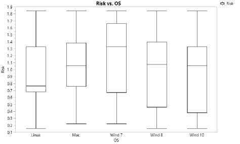
Fig.1. Distributions of the Risk Factors of Operating Systems

Table 4. Means and Variances of Risk Factors for Vulnerabilities in different operating systems.

OS	N (count)	Low	Medium	High	Mean of Risk ^ (R(»j(tj))	Variance of Risk °Z(№j(tj')')
Wind 7	1047	187	278	582	1.1122	0.2668
Wind 8	757	196	209	352	1.0117	0.2946
Wind 10	775	207	249	319	0.9595	0.2748
Linux	2152	457	970	725	0.9038	0.1936
Mac	2107	192	1054	861	1.0987	0.2

According to the results from this method it is observed that, OSs Windows 7 and 10 have the highest mean Risk factors on the date October 30th 2018. Lowest Risk is obtained for Linux. In addition Windows 10 have a significant improvement by having a lower risk factor compared to its previous versions. Next we have to check if there are statistically significant evidence to conclude that mean risk factors are different. We first performed one way ANOVA test to compare the means. It was observed that there are statistically significant evidence for a difference in the mean values. However, as we check for model validity, it was observed that some model assumptions are violated and the model fit is not achieved for the data set. Therefore, we performed NonParametric procedures. Results for both observations are discussed in the next sub sections.

• A.    One Way ANOVA

Our objective is to compare five operating systems for their risk. Considering the set of vulnerabilities discovered and disclosed by the October 30th 2018 is a sample of the entire population of vulnerabilities we can conduct a one way ANOVA to test whether there are any statistically significant differences between the means of two or more independent (unrelated) groups. In our case we will test if there is a statistically significant difference of the “mean risk factor” for vulnerabilities in operating systems considered in this study.

We tested the hypothesis,

H 0 : ^ Rskwn 7 = ^M Riskw„ 8 == M RiskWn i _m = M RskM^c = ^k^

H : at least one of the M_Risk. ' s is different

Result of the F-Test conducted for this hypothesis test is given in Table 05.

Table 5. ANOVA results for five OS

	DF	SS	MS	F-Value	P-Value
Group	4	53.7	13.415	59.06	2.00*E-16***
Residuals	6833	1552.1	0.227

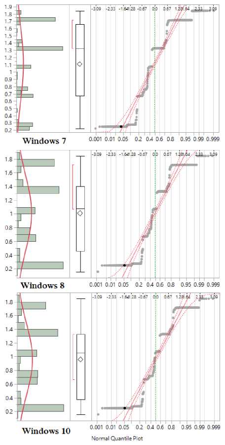
Fig.2. Test for Normality of Windows OS versions

Results of the ANOVA is statistically significant to reject the null hypothesis. The P-Value is very small. Therefore we would reject the null hypothesis and conclude that at-least one of the means of the risk factors is different. However, ANOVA is an omnibus test statistic. Therefore we are still unable to observe which specific groups are statistically significantly different from each other. In other words, we are yet to observe which operating system or systems are significantly different from the others. For this purpose a pair-wise comparison is required. However, before we proceed it is important to confirm if the test is appropriate by checking on ANOVA assumptions.

• B.    ANOVA Assumptions

Validity of the use of ANOVA is based on several assumptions [8]. First, it should be ensured that we have categorical variables grouping a continuous quantitative variable for the response variable. We have five OSs considered here. It should be noted that the risk factor is a product of a “probability measure and an exploitation score which is between 0 and 10 (See equation 11). Therefore, the risk factor is a continuous quantitative variable where the values are truncated between the interval of 0 and 10. As shown in the Box-Plots of the distributions illustrated in the Figure 01, there are no outliers present in any of the distributions. It can also be assumed that the vulnerabilities and exploitation of those vulnerabilities for different operating systems are independent from each other. In addition to these it is important to check for the normality of the distribution of the risk factors and their homogeneity of variances.

To test if the normality condition is satisfied, we start with a group wise Normal Quintile plots given in Figure 2 and Figure 3 . All plots show a significant deviation from the 45 degree reference line of the standardized residuals against the theoretical quantiles of the risk factor values which is also supported by respective Boxplots. This is evidence against the normality assumption. However, ANOVA is a robust methods against the normality violation to some extent. Therefore to further check the normality, we continue to conduct the Shapiro-Wilk normality test. Table 6 illustrates the results of the test.

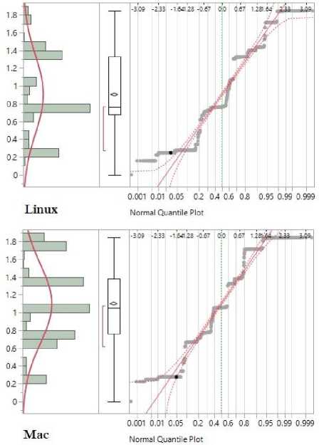
Fig.3. Test for Normality of Linux and Mac OSs

To test the assumption of homogeneity of the variances Bartlett test was conducted and illustrated in Table 6 . Unfortunately, both the conditions are violated significantly.

Shapiro-Wilk normality test results in very low P-Values for distributions of all five operating systems indicating significant evidence against the normality. Similar results were observed in testing for the homogeneity of the variances from Bartlett test. Even though the pare-wise comparison of the Risk factors for five operating systems were conducted by computing Tukey HSD (Tukey Honest Significant Differences) authors move away from parametric procedure and consider Non-Parametric methods due to assumption violations mentioned above.

Table 6. Results of Shapiro-Wilk normality test and Bartlett test of homogeneity of variances

Shapiro-Wilk normality test
OS	Results
Windows 7	W = 0.88849, p-value < 2.2e-16
Windows 8	W = 0.88424, p-value < 2.2e-16
Windows 10	W = 0.89756, p-value < 2.2e-16
Mac	W = 0.94729, p-value < 2.2e-16
Linux	W = 0.92975, p-value < 2.2e-16
Small p value gives evidence against homogeneity of variance.
Bartlett test of homogeneity of variances
Bartlett's     K-squared     =     99.539,     df     =     4, p-value < 2.2e-16
Small p-value gives evidence against homogeneity of variance.

• C.    Non-Parametric Procedure-Kruskal-Wallis test

We proceed with the Kruskal-Wallis test [16] since ANOVA assumptions [8] are not met. The test is an extension of two-sample Wilcoxon test when there are more than two groups. Extracted R outputs are given in the Table 7. For Kruskal-Wallas Chi-squared statistics equals to 181.84, the test resulted in significant very low P-value. This is evidence that the mean risk factors for different OSs are different. However, Kruskal-Wallis test is also an omnibus. Significant P-value only indicates that there are at least two mean risk factors significantly different. Therefore to observe how many such differences are there and which groups are they, we have to conduct a multiple pair-wise comparison between groups by pairwise Wilcox test. In general, using Kruskal-Wallis test we can compare the medians of the different groups which indicates the shift between different groups. However, our data does not support this. As shown in Figure 1, not all five distributions are of the similar shape. There are differences in skewness present. Therefore, we can only compare the mean ranks. Table 8 and Table 9 provide the results of the multiple pairwise comparison obtained by conducting Pairwise Wilcoxon Rank sum test. Wilcoxon rank-sum test is a nonparametric alternative to the two sample t-test which is based solely on the order in which the observations from the two samples fall. To have a pair-wise comparison on five OSs we conduct this test.

Table 7. Kruskal-Wallis rank sum test results

Kruskal-Wallis rank sum test	Kruskal-Wallis chi-squared = 181.84, df = 4, p-value < 2.2e-16
Small p-value gives evidence against homogeneity of variance.

According to the results given in Table 8, there are no statistically significant evidence for a difference of mean risk factors between pairs (Win 8,Win 10), (Win 7, Mac) and (Win 10 and Linux). All other comparisons show significant differences between mean risk factors. To ensure these results further relevant confidence intervals are also obtained and given in Table 9.

For pairs, (Mac, Linux), (Win7, Linux) and (Win8, Linux) we have both positive confidence intervals. This indicated that the mean risk factors of Mac and Windows 7 were significantly higher than the mean risk factor of Linux at the date, October 30th 2018. For pairs, (Win8, Win7), (Win8, Mac), (Win10, Win7) and (Win10, Mac) we have both negative confidence intervals. Therefore, as at October 30th, 2018 the mean risk factor for Win7 was higher than both Win 8 and Win 10. Mean Risk Factor of Mac is also higher than both Win8 and Win 10. Pairs, with confidence intervals having different signs capturing the zero within the interval indicate that there are no statistically significant evidences for a difference in mean risk factors. Therefore results obtained through confidence intervals confirm what is observed through the P-Value.

Table 8. Pairwise Wilcoxon Rank sum test Results with Mean Risk Factors for OS’s

OS	N	Mean of Risk factors M-RvJCtj-y)	Win 7	Win 8	Win 10	Linux
Win 7	1047	1.1122	-
Win 8	757	1.0117	0.00572	-
Win 10	775	0.9595	3.98E-07	0.11737	-
Linux	2152	0.9038	9.92E-22	0.00015	0.40429	-
Mac	2107	1.0987	0.39054	0.00046	8.98E-10	2.40E-38

Table 9. Pairwise Wilcoxon Rank sum test Results with Confidence Intervals.

Level	-Level	p-Value	Lower CL	Upper CL
Mac	Linux	2.4E-38	0.157686	0.285836
Wind 7	Linux	9.92E-22	0.242037	0.311953
Wind 8	Linux	0.000151	0.002335	0.115111
Wind 7	Mac	0.39054	-0.00065	0.003914
Wind 10	Linux	0.40429	-0.00047	0.01579
Wind 10	Win 8	0.117373	-0.02047	3.5E-05
Wind 8	Win 7	0.005722	-0.05078	-0.00017
Wind 8	Mac	0.000456	-0.07028	-0.00118
Wind 10	Win 7	3.98E-07	-0.23773	-0.01828
Wind 10	Mac	8.98E-10	-0.13755	-0.05462

• D.    Interpreting Results

  This study compared the performance of operating systems based on the risk they generated by all reported vulnerabilities over years. So the empirical observation would be to see that higher the mean risk measure, lower the reliability and hence the performance as an efficient and secure operating system. However, the results must not be misinterpreted to compare the overall OS performances at any particular moment. The results we obtained only compare the mean risk factors of all the recorded vulnerabilities which is only one of many useful indicators of the risk aggregated for that operating system created by vulnerabilities discovered and disclosed. More number of vulnerabilities with a higher severity contributes to a higher risk for the OS. We considered the “age” of the vulnerability also hence the probability of exploitation on the date we considered (October 30^th, 2018) is also difference.

However, vulnerabilities after they were found are expected to be patched. Once the patch is introduced and installed, the risk is indeed decreased and a quantitative risk measure should approach zero eventually. If a particular patch attempt fails to fix the vulnerability, such is not considered a successful patch in this study. In addition, a patch for a vulnerability might create another software bug or a vulnerability. In such cases the new vulnerability is considered a different one. However, these complexities in software vulnerability and patch management does not affect our analysis since this study is focused on the threat created by the risk of vulnerabilities until they are fixed actually. In assessing OS performance and comparing them, the patch introduction before and after exploitations occur should also be taken into account. Therefore, developing quantitative measure to assess OS performances is of very complex nature demanding lots of criterion of many varieties. This study is focused on the Mean Risk generated by total number of discovered the vulnerabilities in the OS in the long run. Hence, this is one such method to check the vulnerability risk of any OS.

Mean Risk Factor measure introduced is a quantitative measure that depends on several factors including the time. Therefore, one can calculate the mean risk for different times and observe the behaviour of the mean risk for the same operating system adding new vulnerabilities disclosed in timely manner. Such a study will give more details on the behaviour of the reliability of an operating system through time.

• IV.    Conclusions and Future Works

Assessing OS reliability is a complex task requiring many variables both qualitative and quantitative. Number of vulnerabilities and a measure of their risk assessed quantitatively allow us to compare the risk associated with different OSs. Methodology introduced in the present study enables us to calculate the mean risk of vulnerabilities for an OS at any time given the particular age of the vulnerability till that time (date). Considering only three versions of Microsoft Windows, we observed the mean risk associated decreased significantly for newer versions (especially for Windows 10). There is a statistically significant difference among the mean risk factors of the several operating systems considered. The method can be used with current and future data to assess the mean risk of the OS. Many factors such as users satisfaction, installation simplicity, support for drivers and application software, cost have been used in assessing the performances and reliability of OSs. In addition, number of vulnerabilities and vulnerability response and patch management efficiency are also taken into consideration. Some research efforts have also as mentioned earlier, used forecasting approaches on vulnerabilities and the risk. However, there are no method that consider and use all the past and present vulnerabilities and their associated risk in a time dependant model for each different OSs. This methodology fulfils that necessity in the Cybersecurity related research fields. Using the methodology presented in this study, any researcher can conveniently obtain a quantitative risk measure for any discovered vulnerability as a function of time and then use that to conduct studies in their own research topics and specializations. IT professionals and system administrators also can test this method as an experiment in their network setting with current and future vulnerabilities.