An econometric study of interest rate channel in Russia

Author: Yushina V.A.
Journal: Экономика и бизнес: теория и практика @economyandbusiness
Article in issue: 5-3 (51), 2019.
Free access
Empirical analysis of the interest rate channel of the transmission mechanism of monetary policy in Russia is investigated by applying a vector autoregression model based on monthly data for 2010-2019 under the Taylor rule. The results of the study confirm the presence of statistically significant impact of Bank of Russia’s key rate on the GDP.
Key rate, gdp, inflation, elasticity, transmission mechanism, monetary policy
Short address: https://sciup.org/170181758
IDR: 170181758 | DOI: 10.24411/2411-0450-2019-10749
Эконометрическое исследование процентного канала в России
Эмпирический анализ процентного канала трансмиссионного механизма денежно-кредитной политики в России исследуется путем применения векторной модели авторегрессии на основе месячных данных за 2010-2019 гг. по правилу Тейлора. Результаты исследования подтверждают наличие статистически значимого влияния ключевой ставки Банка России на ВВП.
Text of the scientific article An econometric study of interest rate channel in Russia
Since in recent years the Bank of Russia adheres to the Taylor rule for an open economy, the key rate controlled by it was chosen as an impulse in the models [1].
As mentioned earlier, the vector autoregression VAR method was chosen as a fundamental element of the analysis of the effectiveness of the monetary transmission channels. Vector autoregression is based on the equation of the form:
Vt = Ai * yt_! + иt (N), where y_t and y_(t-1) are the vector of endogenous variables of the corresponding periods,
A_i is a matrix of coefficients, u_t – vector of random disturbances.
The vector of random disturbances can be presented as monetary policy shocks. [2] The analysis of the transparency and clarity of the momentum transfer from monetary policy shocks to the real economy presupposed the choice of the monetary policy instrument, the variables characterizing the financial market, as well as the macroeconomic variable as the ultimate goal of monetary policy, the construction of the VAR model and impulse response functions on the basis of these data [3, 4].
The study estimates the basic second-order vector autoregression model for three time series:
– extrapolated monthly GDP,
– rate of inflation,
– key rate of the Bank of Russia.
The assumption of the model is that the monetary policy shock – the change in the key rate of the Bank of Russia – in the short term has no impact on other variables of the model. All initial data of the model have a monthly dimension, thus being estimated for the period from January 2010 to January 2019.
The main model coefficients and standard OLS statistics are presented in Figure 1. This model approximates real data quite well, since the value of R^(2 ) is close to 1 and the value of a R_adj^2 is close to the value of R^(2 ). S. E. equation is a total measure of regression errors, in this case it tends to 0. Sum sq. resids is also less than any valid value, indicating a high degree of correspondence between the real values and the model. The information criteria of Akaike and Schwartz are also low, so this basic model explains well the real data with a minimum number of free variables. Determinant residual covariance tends to 0, and therefore the evaluation of real data is optimal. The model stability test, which examines the autoregressive roots of a multidimensional time series and displays them on a graph, shows that the time series satisfies the stability condition. The Granger causality test shows that at the 5% significance level, the hypothesis that INFLATION is not the cause of the Granger time series OFF_RATE can be rejected. Thus, we can talk about the change in the key rate of the Bank of Russia as a result of changes in the level of prices in the economy. This conclusion does not apply to other pairs of variables in this model. The test for serial correla- tion of residues showed that there is no serial correlation of any order in the model. According to the white test, p-value is greater than 5% significance level, and therefore the hypothesis of homoscedasticity of residues is not rejected.
The null hypothesis of the test on the normality of residues is rejected, so we can talk about the abnormality of residues.
Vector Autoregression Estimates
Date: 03/31/19 Time: 15:55
Sample (adjusted): 2010M03 2019M01
Included observations: 107 after adjustments
|
GDP |
OFF RATE |
INFLATION |
|
|
GDP(-1) |
1.57724501.. |
. 3.47786264... |
0.00010625... |
|
0.08238120.. |
. 1.26395178... |
6.64668351... |
|
|
[ 19.1457] |
[ 0.27516] |
[ 1.59863] |
|
|
GDP(-2) |
-0.5893311... |
-1.7950470... |
-0.0001027... |
|
0.08293688.. |
. 1.27247736... |
6.69151656... |
|
|
[-7.10578] |
[-0.14107] |
[-1.53554] |
|
|
OFF_RATE(-1) |
8301.47441.. |
. 0.65106708... |
-2.5778688... |
|
7390.15680.. |
. 0.11338510... |
5.96252910... |
|
|
[ 1.12332] |
[ 5.74209] |
[-0.43234] |
|
|
OFF_RATE(-2) |
-6474.4861... |
0.23046691... |
0.06372494... |
|
7066.28369.. |
. 0.10841601... |
5.70122168... |
|
|
[-0.91625] |
[ 2.12576] |
[ 0.01118] |
|
|
INFLATION(-1) |
-331.44500... |
0.00954980... |
0.82020691... |
|
141.719389.. |
. 0.00217436... |
0.11434209... |
|
|
[-2.33874] |
[ 4.39200] |
[ 7.17327] |
|
|
INFLATION(-2) |
23.1966394.. |
. -0.0040482... |
-0.0928541... |
|
134.743818.. |
. 0.00206733... |
0.10871405... |
|
|
[ 0.17215] |
[-1.95822] |
[-0.85411] |
|
|
C |
31161.6454.. |
. -0.5462386... |
27.5540889... |
|
12268.5093.. |
. 0.18823230... |
9.89848334... |
|
|
[ 2.53997] |
[-2.90194] |
[ 2.78367] |
|
|
R-squared |
0.98830973.. |
. 0.86141525... |
0.50230957... |
|
Adj. R-squared |
0.98760831.. |
. 0.85310017... |
0.47244814... |
|
Sum sq. resids |
23958876.9.. |
. 0.00563989... |
15.5962495... |
|
S.E. equation |
489.478058.. |
. 0.00750992... |
0.39492087... |
|
F-statistic |
1409.02092.. |
. 103.596690... |
16.8213528... |
|
Log likelihood |
-810.89402... |
375.187004... |
-48.796210... |
|
Akaike AIC |
15.2877388.. |
. -6.8820000... |
1.04291982... |
|
Schwarz SC |
15.4625967.. |
. -6.7071421... |
1.21777778... |
|
Mean dependent |
19351.2961.. |
. 0.08719626... |
100.566448... |
|
S.D. dependent |
4397.11785.. |
. 0.01959408... |
0.54372275... |
|
Determinant resid covariance (dof adj.) |
1.495280529449659 |
||
|
Determinant resid covariance |
1.220594321545986 |
||
|
Log likelihood |
-466.1438462167166 |
||
|
Akaike information criterion |
9.105492452648909 |
||
|
Schwarz criterion |
9.630066336047975 |
||
|
Number of coefficients |
21 |
||
Figure 1. Descriptive statistics of the model
Source: author calculations
The function of impulse response of the basic VAR-model was evaluated in the framework of the study. Figure 2 shows a clear negative reaction of inflation to monetary policy shocks, while GDP's response to monetary policy shocks is mixed: in the short term, there is a negative reaction, followed by an unexpected positive direction (which may be associated with the approximated monthly value of GDP).
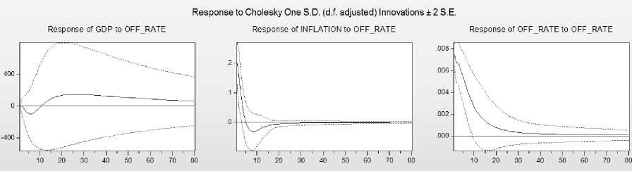
Figure 2. The function of impulse responses in the baseline VAR model Source: author's calculations
References An econometric study of interest rate channel in Russia
- Korhonen I., Nuutilainen R. Breaking monetary policy rules in Russia //Russian Journal of Economics. - 2017. - Т. 3. - № 4. - С. 366-378. - URL: https://www.sciencedirect.com/science/article/pii/S2405473917300594
- Lettau M., Ludvigson S., Steindel C. Monetary policy transmission through the consumption-wealth channel //FRBNY Economic Policy Review. - 2002. - Т. 5. - С. 117-133.
- Esanov A., Merkel C., de Souza L. V. Monetary policy rules for Russia //The Periphery of the Euro. - Routledge, 2017. - С. 159-180.
- Cevik S., Teksoz K. Lost in Transmission? The Effectiveness of Monetary Policy Transmission Channels in the GCC Countries. - 2012.
