An Efficient Switching Filter Based on Cubic B-Spline for Removal of Salt-and-Pepper Noise

Published Online April 2014 in MECS DOI: 10.5815/ijigsp.2014.05.06

When the image is transferred in electronic communication channel, especially in wireless transmission, a noise is considered to be a big common problem and the image will be somewhat changed. In addition, the noise may be corrupted the image during acquisition step, light levels and sensor temperature are the major factors affecting the amount of noise in the resulting images [1],[2]. Image denoising is a very important problem because the quality of image denoising is related to the reliability of all subsequent image processing task. Therefore, the fundamental problem of image processing is to remove the noise while preserving edges and fine details. This paper concentrates on the removal of salt-and-pepper noise, where the noisy pixels can take only the maximum and minimum values in the dynamic range. A large number of methods have been proposed to remove salt-and-pepper noise [3]-[7].

The standard median filter (SM) and its modification such as weighted median (WM) [8] and center weighted median (CWM) [9] are widely used for salt-and-pepper noise elimination. These filters apply the median operation to each pixel without considering whether it is corrupted or not, they tend to alter the noise free pixels as well as the noise pixels, exhibit removing edges and fine details.

To avoid this problem many filter algorithms with noise detectors are proposed such as in the literatures [5],[10]-[13]. However, the major drawback of (SM) is that the filter is effective only at low noise densities when over 50% the details will not be preserved.

In this paper, an efficient filter method is proposed to remove salt –and – pepper noise. In this method, only the noise pixels are changed while the noise free pixels are left unchanged. The cubic B-spline is used as a fitting function to generate additional values within the noise free pixels. The noisy pixel is replaced by the mean value of these pixel values. This method can remove salt-and-pepper-noise with a noise level as high as 97%. Further, this method does not require threshold parameters. The reset of this paper is organized as follows. A brief review of related work and cubic B-spline is given in section II and section III, respectively. In section IV, the proposed method is introduced. The implementation results and comparison are provided in section V. Finally, the conclusions are summed up in section VI.

II RELATED WORK

Many approaches have been proposed to remove salt -and- pepper noise. Haidi et al. [14] have proposed a technique to remove impulse noise from highly corrupted images. The method is actually a hybrid of the adaptive median filter with the switching median filter. The method adaptively changes the size of the median filter based on the approximation of local noise density. Haidi et al [14] claimed that their method is better than the works in [15]-[17]. Abdul Majid and Muhammad Tariq [18] have proposed impulse noise removal scheme that emphasizes on few noise-free pixels. The proposed iterative algorithm searches the noise-free pixels within a small neighborhood. The noisy-pixel is then replaced with the average estimated from noise-free pixels. The iterative process continues until all noisy-pixels of the corrupted image are filtered. In addition, Kenny Kal Vin Toh and Nor Ashidi Mat Isa [10] have proposed a two-stage noise adaptive fuzzy switching median (NAFSM) filter for salt-and-pepper noise detection and removal. Initially, the detection stage will utilize the histogram of the corrupted image to identify noise pixels. These detected “noise pixels” will then be subjected to the second stage of the filtering action, while “noise-free pixels” are retained and left unprocessed. Then, the NAFSM filtering mechanism employs fuzzy reasoning to handle uncertainty present in the extracted local information as introduced by noise. Xuming Zhang and Youlun Xiong [19] have proposed two-stage algorithm, called switching-based adaptive weighted mean filter to remove salt-and-pepper noise from the corrupted images. First, the directional difference based noise detector is used to identify the noisy pixels by comparing the minimum absolute value of four mean differences between the current pixel and its neighbors in four directional windows with a predefined threshold. Then, the adaptive weighted mean filter is adopted to remove the detected impulses by replacing each noisy pixel with the weighted mean of its noise-free neighbors in the filtering window. Furthermore, a modified decision based unsymmetrical trimmed median filter algorithm (MDBUTMF) for highly corrupted image by salt -and- pepper noise is proposed in [13]. This algorithm replaces the noisy pixel by trimmed median value when other pixel values, 0’s and 255’s are present in the selected window and when all the pixel values are 0’s and 255’s then the noise pixel is replaced by mean value of all the elements present in the selected window. In addition, K. S. Srinivasan and D. Ebenezer [12] have proposed a decision-based algorithm (DBA) for restoration of images that are highly corrupted by impulse noise. This method processes the corrupted image by first detecting the impulse noise. The detection of noisy and noise-free pixels is decided by checking whether the value of a processed pixel element lies between the maximum and minimum values that occur inside the selected window. This is because the impulse noise pixels can take the maximum and minimum values in the dynamic range (0, 255). If the value of the pixel processed is within the range, then it is an uncorrupted pixel and left unchanged. If the value does not lie within this range, then it is a noisy pixel and is replaced by the median value of the window or by its neighborhood values. Cangju Xing [6] has proposed a method to remove salt-and-pepper noise. This method includes three steps. In the first step, the noise pixels are distinguished from the signal pixels; then set initial values for noise pixels; finally, compute the output. The main difference from other switch-type filters is the means to change the values of the contaminated noise pixels.

III CUBIC B-SPLINE

When approximating functions for fitting measured data, it is necessary to have classes of functions which have enough flexibility to adapt to the given data, and which, at the same time, can be easily evaluated on a computer. Traditionally polynomials have been used for this purpose. These polynomials have some flexibility where they can be computed easily. However, for rapidly changing values of the function to be approximated the degree of the polynomial has to be increased, and the result is often a function exhibiting wild oscillations. The situation changes dramatically when the basic interval is divided into subintervals, and the approximating or fitting function is taken to be a piecewise polynomial. That is, the function is represented by different polynomials over each subinterval. The polynomials are joined together at the interval endpoints (knots) in such a way that a certain degree of smoothness (differentiability) of the resulting function is guaranteed. If the degree of the polynomials is k , and the number of subintervals is n + ¹ the resulting function is called (polynomial) spline function of degree k with n knots.[20]-[21]

A B-spline is a sufficiently smooth polynomial function that is piecewise- defined, and possesses a high degree of smoothness at the places where the polynomial pieces connect (which are known as knots). It used in many applications such as interpolation and data fitting. Forever, B-splines are used on graphics applications to design curve and surface shapes, to digitize drawings for computer storage, and to display animation paths. B-spline functions have useful properties such as smooth, flexible and easy to store and manipulate on a computer. For this, cubic B-spline is developed for salt-and-pepper noise removal.

Cubic B-splines are very common, as they provide a geometry that is one step away from simple quadratics, and possess continuity characteristics that make the joins between the segments invisible. Given the points (xо, У0) to (xn , У. ) where  x0 < x, < .... < x. so we write the n cubic polynomial pieces as

S i⁽ x ) = a i + b i ⁽ x - x i ) + c i ⁽ x - x i )² + d i ( x ^— x i )³           (1)

Each ⁱ has four unknowns ( aⁱ , ⁱ , cⁱ , ⁱ ) and i   0,... n  1 . So, there are a total of 4 . unknowns.

h = x , — x.

It is very helpful to introduce the 1     1+1     1. Then the spline conditions can be written as follows [22]:

a = Vi

a ,. + hb + h² c_: + h ³ d = y^,                (3)

i          i i          i i          i i           i +1                                             ' ^

b + 2 hc + 3 h 2 d - b ₁₊,= 0                (4)

2 c + 6 hd - 2 c _/+, = 0                      (5)

The equations from (2) to (5) can be written as large linear system for 4 n the unknowns as follows [22].

[ a 0 , b o , c ₀ , ^d 0 , a l , b l , ^C 1 , d i ,..., a n - 1 , b n - 1 , ^c n - 1 , d n - 1 f

IV PROPOSED METHOD

Noise detection is the first stage in this method. The salt-and-pepper noise pixels can take the maximum and minimum values in the dynamic range. Therefore, if the value of the processing pixel lies between the 0 and maximum value of the dynamic range inside the window, then it kept unchanged. If the value does not lie within this range, then it may be noisy pixel and it is replaced by the output of the filter operation.

In noise cancellation stage, the window size is changed according to the local noise density. Only switching between 3x3 and 5x5 window size is used in order to less the blurring effect. The noise-free pixels are only considered in the filter operation to evaluate the new value of the processing pixel. If all the pixels in the 3x3 window are considered to be noisy, then the filter window is switched to 5x5. If all the pixels inside the 5X5 window are noisy, then replace the processing pixel by the previous resultant pixel. Cubic B-spline is used to generate additional value with noise free pixel inside the window. The mean value of all these pixels is the value of the processing pixel. The values of h in cubic B-spline functions are based on the number of noise-free pixels inside the window. The proposed method is summarized and described by the following algorithm. In addition, the flowchart diagram is shown in Fig.1.

Step 1: Select 2-D window of size 3x3 and the pixel P being processed is ^ij .

0 <  p <  255     P

Step 2: If         ^ij         then ^ij is noise-free pixel

P and its value is left unchanged; go to Step 1 for next ij

Step 3: If the window contains all the elements as 0’s and 255’s. Then go to Step 6.

tep 4: If only one pixel value inside the window not

P equal to 0 and 255. Then replace ij with this pixel

P value; go to Step 1 for next ij

Step 5: If the window contains two or more pixel values not as 0’s and 255’s.

• 5.1    Eliminate 255’s and 0’s

• 5.2    Use a cubic B-spline to generate additional values with the remaining noise free pixels where

• 5.3    Replace ^ij with the mean value of all these

h takes 0.1, 0.05 or 0.01 if the number of the noise free pixels are large than or equal 4, equal 3 or equal 2, respectively.

P

P values; go to Step 1 for next ij

Step 6: Increase the window size by 5X5.

Step 7: If the window contains all the elements as 0’s

P and 255’s. Then replace ij by the previous resultant pixel.

Step 8:If only one pixel value inside the window not

P equal to 0 and 255. Then replace ij with this pixel

P value; go to Step 1 for next ij

.

Step 9: If the window contains two or more pixel values not as 0’s and 255’s.

• 9.1    Eliminate 255’s and 0’s

• 9.2    Use a cubic B-spline to generate additional values with the remaining noise free pixels where h takes 0.15, 0.1, 0.05 or 0.01 if the number of the noise free pixels are large than or equal 5, equal 4, equal 3, or equal 2, respectively.

• 9.3    Replace ^ij with the mean value of all these

P

P values; go to Step 1 for next ij

V SIMULATION RESULTS

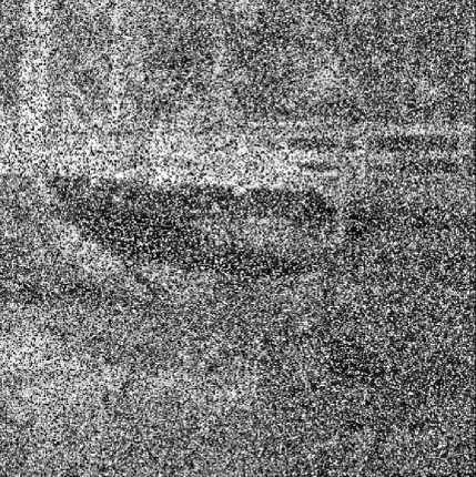
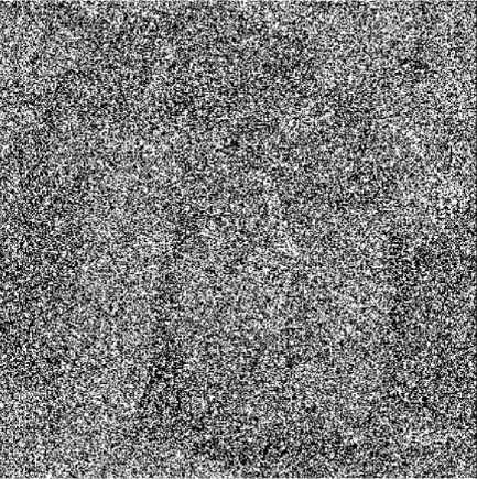
The performance of the proposed method is tested with 1024x1024 different grayscale images such as Bridge, Peppers and Ships with their dynamic range values of [0,255]. The noise densities are varied from 10% to 97%, and restoration performances are quantitatively measured by peak signal-to-noise ratio (PSNR) as defined in (7)

PSNR = 10log₁₀

' (255) 2 ' _v MSE ,

^L ( F ( i , j ) - F¹ ( i , j ) ) 2

MSE = j^----------

M x N

where MSE stands for mean square error, ^{M x N} is size of the image, F represents the original image and ^F denotes the denoised image. The standard median filter (SMF), Haidi et al method [14], Abdul Majid and Muhammad Tariq method [18] and MDBUTMF method [13] are adopted to make comparison with the proposed method (PM). Table I, Table II and Table III show PSNR value of (PM) against the existing methods by varying the noise density from 10% to 97% for

Bridge, Peppers and Ships images, respectively. Thus, it can be seen that the PM produces higher PSNR values than other methods. In addition, Fig.2, Fig.3 and Fig.4 show a plot of PSNR versus noise densities for Bridge, Peppers and Ships images, respectively. The visual result of the proposed method for Bridge image corrupted by 50%, Peppers image corrupted by 80% and Ships image corrupted by 97% are shown in Fig.5, Fig.6 and Fig.7, respectively.

Table I: COMPARISON OF PROSSING RESULTS IN PSNR (dB) FOR BRIDGE IMAGE.

Noise density	SMF	Method [18]	MDBUTMF [13]	Haidi [14]	PM
20 %	29.3538	50.7	48.3236	36.1801	50.4049
30 %	23.9478	47.6130	44.7659	33.9602	47.3144
40 %	19.1396	44.5466	41.2087	32.6065	44.7039
50 %	15.2561	41.4843	36.3076	31.4620	42.5042
60 %	12.2568	37.8147	30.4300	29.9041	40.3174
70 %	9.9091	33.548	24.9938	27.7907	38.2771
80 %	7.9927	28.7064	19.8859	25.9067	35.7651
90 %	6.4850	19.7134	15.3091	23.3135	31.0357
95 %	5.8551	5.8362	13.2396	21.0217	26.3168
97 %	5.6152	5.5167	12.4492	19.6282	23.0645

Table II: COMPARISON OF PROSSING RESULTS IN PSNR (dB) FOR PEPPERS IMAGE.

Noise density	SMF	Method [18]	MDBUTMF [13]	Haidi [14]	PM
20 %	30.5085	53.4157	51.1776	36.9457	53.3864
30 %	24.4380	50.0587	47.2928	34.6169	50.0888
40 %	19.2232	46.8962	43.0239	33.4325	47.3528
50 %	15.3275	43.8037	37.0994	32.2007	44.8572
60 %	12.3661	39.8965	31.1429	30.6334	42.6822
70 %	9.9594	34.7032	24.7732	28.6588	40.5849
80 %	8.0579	29.4274	19.9782	26.6614	38.0008
90 %	6.5276	19.8039	15.5061	24.0642	33.1538
95 %	5.8868	5.6098	13.4513	21.8485	27.1668
97 %	5.6543	5.3078	12.6471	20.3038	23.7474

Table III: COMPARISON OF PROSSING RESULTS IN PSNR (dB) FOR SHIPS IMAGE .

Noise density	SMF	Method [18]	MDBUTMF [13]	Haidi [14]	PM
20 %	29.2870	50.5787	48.2574	37.2386	50.1887
30 %	23.9724	47.4498	44.9186	34.6722	47.0900
40 %	19.3251	44.6286	41.6909	33.0803	44.6110
50 %	15.5374	41.7571	37.0550	31.8681	42.3243
60 %	12.4728	38.2494	31.4745	30.4524	40.1992
70 %	10.0703	34.1994	26.0011	28.3868	38.0876
80 %	8.2138	28.7160	20.8025	26.4371	35.7502
90 %	6.6895	20.1565	16.2866	23.7247	31.2785
95 %	6.0545	5.9649	14.2113	21.4844	26.3710
97 %	5.8151	5.6668	13.3714	20.0054	22.9994

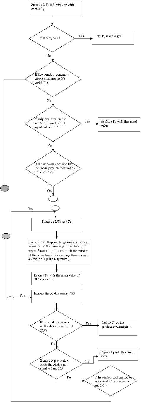
Figure 1. The flow chart of the proposed method

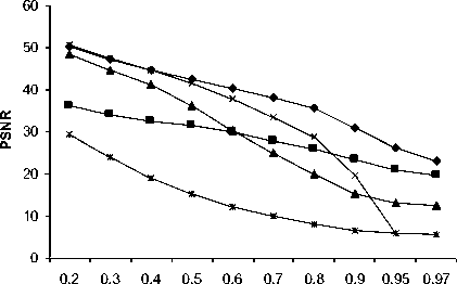
—♦— PM              Haidi [14]     —*— MDBUTMF [13]

Method [18]         SMF

Figure 2. Comparison graph of PSNR at different noise densities for Bridge image.

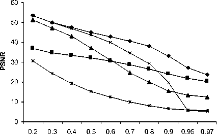
—♦— PM              Haidi [14]     —*— MDBUTMF [13]

Method [18]         SMF

Figure 3. Comparison graph of PSNR at different noise densities for Peppers image.

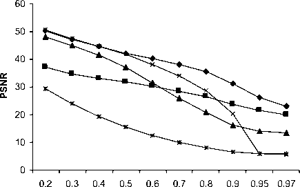
—♦— PM                 Haidi [14]       ▲ MDBUTMF [13]

Method [18]        SMF

Figure 4. Comparison graph of PSNR at different noise densities for ships image.

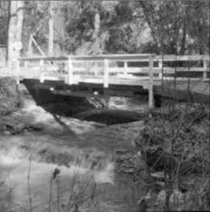
(a) Original image

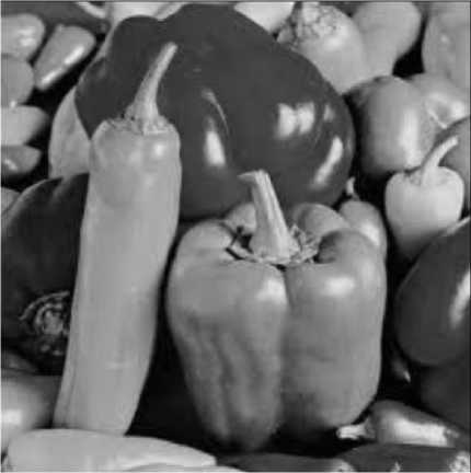
(a) Original image

(b) Corrupted image by 50%

(b) Corrupted image by 80%

(c) Processed image

Figure 5. The result of PM for corrupted Bridge image by 50%

(c) Processed image

Figure 6. The result of PM for corrupted Bridge image by 80%

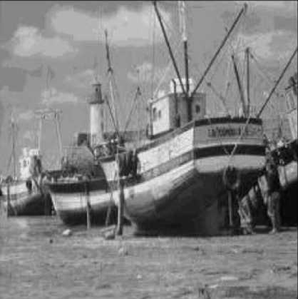
(a) Original image

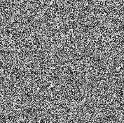
(b) Corrupted image by 97%

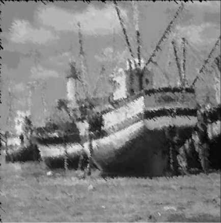
(c) Processed image

Figure 7. The result of PM for corrupted Bridge image by 97%

VI CONCLUSION

This paper presents a novel method to remove salt-and-pepper noise from highly corrupted images. This method does not need the threshold parameter. Thus, no tuning or training is required. Furthermore, the filter size is adaptable to the local noise density. This filter shows consistent and stable performance across a wide range of noise densities where the effective noise removal can be observed even up to 97%. The framework of this method outperforms other existing denoising methods for removal of salt - and - pepper noise with preserving image details as it is clearly seen in visual and quantitative results.