An efficient texture feature extraction algorithm for high resolution land cover remote sensing image classification

Published Online December 2018 in MECS

Image segmentation and image classification are significant tasks in any remote sensing image analysis. Classified land cover or land use remote sensing images have various socio, economic and environment applications like agriculture monitoring, urban planning, forest monitoring, change detection, forest fire detection, detection and monitoring of volcanoes, road extraction, river extraction, monitoring of ocean ridges, etc [1, 2, 3, 4, 5, 6, 7, 8]. Many techniques have been proposed in the literature for the classification of a high resolution remote sensing image. Few of them include pure pixel-based techniques, techniques involving mathematical morphology, seed growing techniques,  watershed algorithms, wavelets, Markov random fields, Grayscale co-occurrence matrices, neural networks, graph theory, etc [9, 10, 11, 12, 13, 14, 15]. Classification techniques involving only single pixel values may not perform well always as the spatial context is missing. Many texture feature extraction algorithms are mentioned in literature [12, 16, 17, 18], with the help of which the spatial parameter also could be considered along with the pixel values.

Mathematical morphology suits very well for remote sensing images and was a proved tool for featuring textured objects [2, 3, 4, 5, 13, 19, 20, 21, 22, 23]. Also, any digital image could be considered as a random closed set and contact distributions are tools which are used to describe the distributional properties of random spatial structures from outside the structure [24,   25].

Distributions to the first contact for increasing test sets contained in the void are called as contact distributions and can be very well used for exploratory data analysis of random patterns [25]. If the test set or structuring element is a line segment, those contact distributions are called as linear contact distributions. In this paper, a new algorithm "Linear Contact Distributions and First Order Statistics Classification Algorithm" (LCDFOSCA) has been proposed. In this algorithm, texture features of every pixel are extracted with the help of mathematical morphology [13, 14, 26], linear contact distributions (LCD) [24, 25] and first-order statistics (FOS) [27]. The texture features thus extracted are clustered with the help of the K-means clustering algorithm and finally, the classified image could be displayed.

Paper is organized as follows. Section 2 deals with methodology, section 3 presents results and discussions and section 4 concludes the paper with the discussion of future scope.

• II. Methodology

Irene Epifanio and Pierre Soille have proposed a supervised texture feature algorithm [28] to segment a remote sensing image using LCD. Here, some training set is required to segment the image as the features extracted cannot be clustered as they do not converge with any clustering algorithm. Hence, a new unsupervised algorithm LCDFOSCA was proposed in this paper which calculates features for every pixel and later all these features could be clustered even with the k-means algorithm. No training set is required to classify the image.

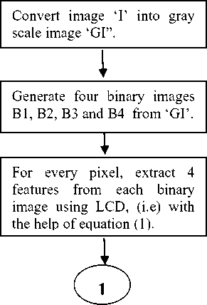
The flow of the algorithm is explained in the flowchart as given in Fig.1.

Read the true color satellite image ‘I’.

I

Display the classified image

I

Fig.1. Flowchart of methodology.

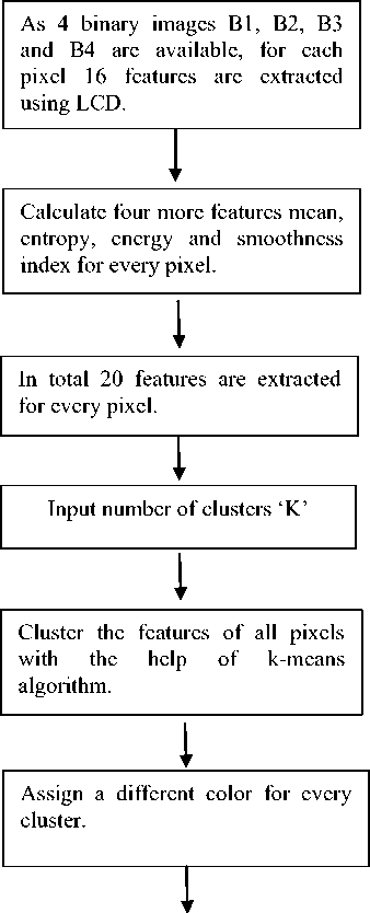
Initially the given image 'I' is converted into a grayscale image 'GI'. From this grayscale image 'GI', to enhance the textural properties, four binary images B1, B2, B3, and B4 are extracted. From each binary image, and for every pixel, four features are extracted with the help of LCD. As 4 binary images are available, 16 features are extracted for each pixel. Similarly, four more features are extracted for every pixel using FOS. Thus in total 20 features are extracted for every pixel. After completing extracting 20 features for all the pixels in the image, these feature vectors are classified using the k-means algorithm and are finally classified. The process of generation of binary images and extraction of texture features is explained in more detail in the coming sections.

• A.    Generation of binary images

In this paper, prior to calculating LCD’s of every pixel, the given image is converted into four binary images to highlight the texture patterns present in the image [28,31]. For this purpose,

• (1)    Initially, the given image ‘I’ is converted into a grayscale image ‘GI’.

• (2)    From image ‘GI’, two threshold values ‘th1’ and ‘th2’ are to be estimated.

• (3)    To estimate the value ‘th1’, first estimate a value ‘th’ from image ‘GI’, with the help of OTSU method [29, 30]. Multiply ‘th’ with maximum intensity value ‘255’ to get ‘th1’ [31].

• (3)    With the help of th1, the grayscale image ‘GI’ is converted into binary image ‘BIM’, by thresholding image ‘GI’ with value ‘th1’. All values less than ‘th1’ in image ‘GI’ are taken as ‘1’ and remaining as ‘0’ to get the binary image ‘BIM’.

• (4)    To calculate the second threshold value ‘th2’, generate external gradient image ‘EI’ from ‘GI’ with a flat 3 x 3 structuring element with value ‘1’. Threshold ‘th’ is estimated from ‘EI’ with the help of OTSU method [29, 30, 31]. Multiply ‘th’ with maximum intensity value 255 to get the threshold ‘th2’ [31].

• (5)    Now external gradient images ‘EG1’, ‘EG2’, EG3’ and ‘EG4’are obtained from image ‘GI’ with structuring elements S1, S2, S3, and S4.

• S1    is the structuring element with a diamond of radius 7,

• S2    is the structuring element with a disc of radius 7,

• S3    is the structuring element of a square with side 11 and

• S4    is the structuring element of the cross with arm ‘5’.

• (6)    Thresholded external gradient images ‘TEG1’, ‘TEG2’, ‘TEG3’ and ‘TEG4’ are obtained from external gradient images ‘EG1’, ‘EG2’, EG3’ and ‘EG4’ with the help of threshold ‘th2’. All values greater than ‘th2’ are taken as ‘1’ and remaining as ‘0’ to get the thresholded external gradient images.

• (7)    Thresholded external gradient images ‘TEG1’, ‘TEG2’, ‘TEG3’ and ‘TEG4’ are now intersected with binary image ‘BIM’ to get four intersected images.

• (8)    Final binary images ‘B1’, ‘B2’, ‘B3’ and ‘B4’ are obtained by area opening four intersected images with value 10.

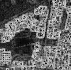
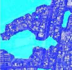
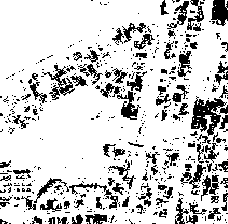
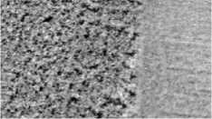
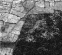
Fig.2 shows various intermediate results of the process. Fig.2a is the original true color image from ‘Tirupathi’ area dataset. Fig.2b is the panchromatic image on which the algorithm has been applied, Fig.2c is the thresholded binary image ‘BIM’, Fig.2d is one of the four external gradient images generated ‘EG1’, Fig.2e is one of the four final intersected and area opened binary images generated ‘B1’ and Fig.2f shows the final classified image.

(b)

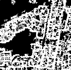
Fig.2. Classification results for proposed algorithm LCDFOSCA (a) True color image (b) Panchromatic image (c) Thresholded image with threshold 'th1'(d) External gradient image (e) Intersected and area opened binary image (f) Final Classified image

(d)

(f)

(a)

• B.    Extraction of texture features

Linear contact distributions of any pixel can be estimated with the help of Equation (1) [24, 28, 32]. To estimate LCD of a pixel, a window ‘W’ of size n x n is considered surrounding the pixel under consideration. If ‘C’ is the set of pixels with value one in window ‘W’, then the LCD for a line segment with length ‘L’ and angle ‘ɵ’ is given by

H ^θ ( L ) = 1 -

A ( ε S ( L , θ ) ( C ) ^c ). A ( W )

A ( ε S ( L , θ ) ( W )). A (( C ) ^c )

Where εB(A) denotes erosion of set ‘A’ by set ‘B’. Also, S(L, ɵ) is a structuring element, which consists of a line segment with length ‘L’ and angle ɵ. (C)c represents the complement of set “C”. ‘A’ is the area, here calculated as a number of pixels. In this paper, the length of the line segment has been considered as 3 and for every pixel, LCD’s are estimated in all four principal directions. That is, the structuring elements considered are as follows.

	"0	0	0"		" 0	1	0 "
S 1 =	1	1	1	S 2 =	0	1	0
	0	0	0 .		0	1	0 .
	"0	0	1"		" 1	0	0"
S 3 =	0	1	0	S 4 =	0	1	0	(2)
	. 1	0	0		. 0	0	1 .

From each binary image, for every pixel ‘p’, LCD are calculated with the help of equation (1) and structuring elements presented in equation (2), to get four features for the pixel. As four binary images are available and from each binary image, a pixel gets 4 features, every pixel will get 16 features. From the grayscale image ‘GI’, four more features are calculated for every pixel, with the help of first order statistics mean, entropy, smoothness index, and energy [27]. They are calculated for the window ‘W’, surrounded by the pixel considered. Hence for every pixel, 20 features are calculated.

Algorithm to calculate the feature vector for every pixel:

Input: Binary images B1, B2, B3, B4 and grayscale image GI.

Output: Feature vectors for all the pixels of the given image.

Assume the size of the image to be r x s.

• (1)    Consider the binary image B1.

• (2)    Let structuring element is S1 as given in equation.(2).

• (3)    For i = 1 to r

• (4)    For j = 1 to s

• (5)    Consider a window ‘W’ of size n x n surrounding the pixel p(i,j).

• (6)    Calculate the feature f1 from window ‘W’ using equation (1).

• (7)    Repeat step 6 with structuring elements S2, S3 and S4 as given in equation.(2) to get the features f2, f3 and f4 for pixel p(i,j).

• (8)    Repeat from step 5 to step 7 with binary image B2, B3 and B4 to get features f5 to f16.

• (9)    From grayscale image ‘GI’, consider the window ‘W1’ of sixe n x n surrounding the pixel p(i,j).

• (10)    Calculate other features f17 to f20 from window ‘W1’ like mean, entropy, smoothness index and energy.

• (11)    end of for loop of j.

• (12)    end for loop of i.

(13)stop.

• C.    Classification of the image

All feature vectors calculated for every pixel are stored in a file and are clustered with the help of the K-means algorithm. All pixels of the first cluster are allotted one color, pixels of the second cluster are allotted another color and so on. Finally, all pixels are displayed thus forming a classified image.

• III.    Results and Discussions

• A.    Experimental setup

The algorithm has been applied on various true color images of NRSC ‘Tirupathi’ region [33] and on Google Earth images [34]. Small portions of the satellite image are cropped with the help of ‘QGIS’, an open source software and algorithm is applied on those cropped images. Cropped images of various sizes are considered. All algorithms are implemented in ‘MATLAB’. The window size of 51 x 51 is considered to calculate the feature vectors of every pixel. All ground truth images are generated manually by visually interpreting the true color images.

• B.    Datasets

• 1.  2.5m Color satellite image of NRSC (National

• 2.    1m Color satellite image of NRSC ‘Tirupathi and western side of Tirupathi’ region covering NARL, Chittoor, Andhra Pradesh, India. Latitude and longitudes of the left top corner and right bottom corners are (13.70⁰, 79.11⁰) and (13.60⁰, 79.46⁰) [33].

• 3.    Google Earth image of ‘Kollipara’ region of Andhra Pradesh state with latitude 16.283197⁰ and longitude  80.775660⁰.  Eye alt at 755ft and

  acquired on 19-10-2017 [34].

Remote Sensing Center) ‘Tirupathi and western side of Tirupathi’ region covering NARL, Chittoor, Andhra Pradesh, India. The site contains water bodies, urban, forests, etc. Latitude and longitudes of the left top corner and right bottom corners are (13.700, 79.110) and (13.350, 79.460) [33].

• C.    Result analysis

Both subjective and quantitative analyses have been performed for evaluating the proposed algorithm. Both have proved the efficiency of the proposed algorithm. It has also been proved that LCDFOSCA was able to classify various land cover images without the help of any training data.

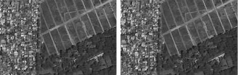
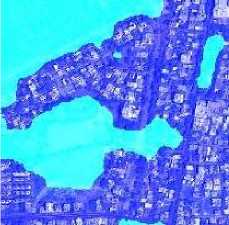
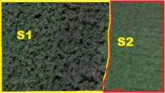
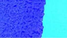
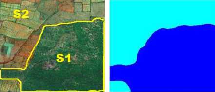
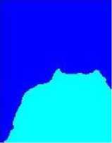
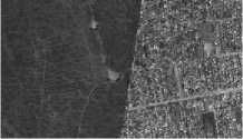
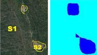
Fig.3, Fig.4, Fig.5, Fig.6, Fig.7, Fig.8, and Fig.9 present some of the results for the algorithm LCDFOSCA. Fig.3a is a cropped image from ‘Tirupathi’ area data set and Fig.3b is the grayscale image on which the algorithm is applied. Fig.3c is the ground truth and Fig.3d is the final segmented image with the help of LCDFOSCA algorithm. The dark blue region of the classified images represents the built-up area and cyan color region represents the vegetation.

(a)                                    (b)

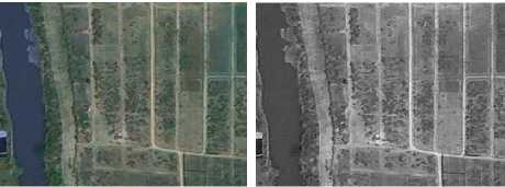
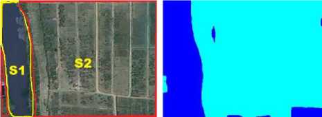
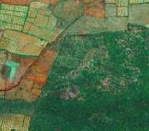
Fig.4a is a Google Earth image with the patterns of two types of crops. Fig.4c is the ground truth and Fig.4d is the classified image, which has rightly classified two types of crops. Fig.7a is also a ‘Tirupathi’ area true-color satellite image with 2mts resolution. LCDFOSCA has classified the original image into two clusters, forest region, and cultivated region. It is very near to the ground truth.

(a)                                    (b)

(c)                                    (d)

(c)

(d)

Fig.3. Buildings and trees: Classification results for proposed algorithm LCDFOSCA (a) True color image (b) Panchromatic image (c) Ground truth image (d) Classified image

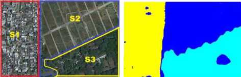
Fig.5. Buildings, trees and crops: Classification results for proposed algorithm LCDFOSCA (a) True color image (b) Panchromatic image (c)

Ground truth image (d) Classified image

(a)                                    (b)

If Fig.4 and Fig.7 are observed, it could be noted that, if the image at a macro scale is given, LCDFOSCA algorithm was able to segment the image into various land use, like forest region and cultivated lands region. But, if an image with micro scale is given, for example:

(c)                                    (d)

(a)

(c)

(d)

(a)

Fig.6. River and trees: Classification results for proposed algorithm LCDFOSCA (a) True color image (b) Panchromatic image (c) Ground truth image (d) Classified image

(b)

Fig.4. Two types of crops: Classification results for proposed algorithm LCDFOSCA (a) True color image (b) Panchromatic image (c) Ground truth image (d) Classified image.

(c)                                    (d)

Fig.7. Cultivation and forest: Classification results for proposed algorithm LCDFOSCA (a) True color image (b) Panchromatic image (c)

Ground truth image (d) Classified image

(a)                                    (b)

(c)

(d)

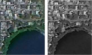
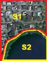
Fig.8. Water and buildings: Classification results for proposed algorithm LCDFOSCA (a) True color image (b) Panchromatic image (c) Ground truth image (d) Classified image.

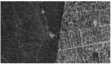
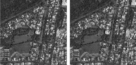
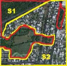
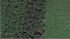
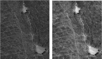
Fig.4, the algorithm is able to classify various types of crops. Fig.5, Fig.6, Fig.8, and Fig.9 are all images from "Tirupathi" area 1mt resolution. If the final classified images are observed, we can easily find that they are very much nearer to their respective ground truths. LCDFOSCA was able to classify water, buildings, forest, cultivation lands, various types of crops, etc from the images. Fig.10 is a part clipped from Fig.9. When LCDFOSCA was applied on Fig.9, and was asked to classify into two groups, it classified the image into "buildings" class and "forest" class as seen in Fig.9d. But, when LCDFOSCA was applied on the Fig.10a, which is a part of Fig.9a, it classified the image as ‘trees’ and empty’ regions. Hence, LCDFOSCA is able to cluster the images into various parts unsupervised depending on the scale of the image. As a neighborhood window is being considered, the border effect could be observed sometimes. For example, Fig.6 shows this border effect. By observing ground truth and classified pictures Fig.6c, and Fig.6d respectively, the difference could be found easily near the banks of the river.

(c)

(d)

Quantitative analyses of the results are performed using the Dice coefficient, Jaccard coefficient, Precision, Sensitivity, Specificity and segmentation accuracy [35, 36, and 37]. If Dice coefficient value is greater than 0.70, the segmentation is said to be good [38]. Table 1. shows the performance results of all the said measures. Dice coefficient of all segments of all the images is more than 0.85, and for most of the images, it is greater than 0.95, which shows that the results are good. Segmentation accuracy of all images is greater than 0.75 and Jaccard coefficient is greater than 0.90 for most of the images.

• IV.    Conclusion

  Fig.9. Buildings and forest: Classification results for proposed algorithm LCDFOSCA (a) True color image (b) Panchromatic image (c) Ground truth image (d) Classified image.

  

  (a)                                    (b)

  
  
  

  (c)                                    (d)

  Fig.10. Trees clip: Classification results for proposed algorithm LCDFOSCA (a) True color image (b) Panchromatic image (c) Ground truth image (d) Classified image.

  
  

In this paper a new unsupervised algorithm, LCDFOSCA has been introduced to extract texture features for classification of a remote sensing image. LCDFOSCA is able to classify almost all land cover images which include water, forest, buildings, cultivation lands, various types of crops, etc. Both subjective and quantitative analyses are performed for the said algorithm. The subjective analysis shows that the algorithm performs well for classifying various objects of the remote sensing images and is also able to segment very similar and close patterns too. It also proved that the algorithm is able to classify a macro scale or a microscale image. Quantitative analysis shows that the dice coefficient values are greater than 0.85 for all images and for most of them it is greater than 0.95. Segmentation accuracy values range from 0.76 to 0.99 and Jaccard coefficient values are greater than 0.90 for most of the segments. In LCDFOSCA, the simple k-means algorithm is used to cluster the texture features of the image. More robust techniques like fuzzy c-means, rough sets, soft sets, etc could be tried in the future for further improvement of the clustering efficiency and thus finally the classification efficiency of the image. Border effects could be observed in the resultant images, sometimes as texture features are estimated in a neighborhood window of the pixel. Hence, the future scope of work could also include solving border effects.

Anyhow, features extracted with LCDFOSCA are very good as they performed well even with a simple k-means clustering algorithm.

Table 1. Performance Evaluation

S.no	Name  of  the image	Segment	Dice coefficient	Jaccard Coefficient	Segmentation accuracy	Precision	Sensitivity	Specificity
1	Buildings    and trees	S1	0.9458	0.8716	0.7611	0.8853	0.7280	0.8070
		S2	0.9944	0.9820	0.9812	0.9955	0.9863	0.9936
2	Two  types  of crops	S1	0.9911	0.9668	0.7799	0.9689	0.7339	0.9297
		S2	0.9860	0.9386	0.8417	0.9749	0.7121	0.9758
3	Cultivation   and forest	S1	0.9684	0.9247	0.7944	0.9723	0.7039	0.9097
		S2	0.9639	0.9009	0.8137	0.9490	0.6924	0.9281
4	River and trees	S1	0.8562	0.6754	0.7840	0.6754	0.5956	0.8883
		S2	0.9737	0.9219	0.5899	1.0000	0.5694	1.0000
5	Water      and buildings	S1	0.9860	0.9458	0.8022	0.9554	0.7305	0.9575
		S2	0.9812	0.9246	0.8569	0.9305	0.7347	0.9613
6	Buildings,   trees and crops	S1	0.9976	0.9947	0.9968	0.9999	0.9949	0.9994
		S2	0.9737	0.9466	0.9798	0.9665	0.9801	0.9839
		S3	0.9877	0.9749	0.9894	0.9909	0.9839	0.9944
7	Buildings    and forest	S1	0.9999	0.9957	0.8679	0.9978	0.8497	0.9937
		S2	0.9988	0.9943	0.8384	0.9958	0.8429	0.9901