An environment aware learning-based self-adaptation technique with reusable components

Published Online June 2019 in MECS DOI: 10.5815/ijmecs.2019.06.06

In this era of intelligent computing, the operating environment of software systems has become more complex. Due to the ever-dynamic nature of these systems, goals may be violated at any time. For example, the maximum 3s response time goal of a system may be violated if the number of users exceeds a predefined threshold. In this situation, manual operations can be carried out to increase the system service level [1]. For instance, more servers can be added along with a load balancer to bring back the system in its goal conforming state. However, as there can be large number of goals, detecting goal violations and applying fixes manually are inefficient. Therefore, self-adaptive systems that automatically satisfy goals at runtime are essential.

Machine learning techniques are widely used for data-driven automated decision making. These are applicable where static condition-action rules are insufficient. For self-adaptive systems, a large number of condition-action rules are required to support numerous goals and goal violation conditions [2]. Furthermore, these rules need to be altered when goals or the dynamics of the environment change. Due to this, machine learning can be applied to build effective self-adaptive systems. Although this reduces the effort of manual construction, the reusability of self-adaptation managers that control self-adaptation can further minimize this effort.

Kim et al. proposed a reinforcement learning based approach to self-adaptation. They modeled self-adaptive systems as a Markov Decision Process and used Q-learning for action selection [3]. Ho et al. proposed a self-adaptive technique where a model of the environment was learned using supervised learning [4]. This model was used to calculate the value function which helped to construct the action selection policy. Nevertheless, reinforcement learning techniques are computationintensive when the number of state-action pairs is large. Hence, supervised learning based approaches emerged. The FUSION approach proposed by Esfahani et al. is a supervised learning based technique for self-adaptation [5, 6]. FUSION defined a regression equation to express system metrics as a combination of features. Features are variation points of the system which are subset of the system architecture. In FUSION, feature maps to the individual modules of the system which can be swapped at runtime [5, 6]. The feature-metric equations are used to maximize the total utility of the system which is expressed as a function of the system metrics. The concept of feature is the core of FUSION. Apart from the internal features of the system, the metrics can be dependent on external environmental features (e.g., request rate, service time etc.) which FUSION did not consider. It further did not address reusability. However, as reuse reduces effort, it should be enforced to be inherently present in a self-adaptive approach.

This paper proposes a learning-based self-adaptation technique with built-in reuse potential. The main contributions of this paper are as follows.

• •    The notion of feature from FUSION model is changed to variant. A variant is any variation point in a system such as software components and environmental factors. A structured learning-based self-adaptation technique using these variants is presented. The data required for learning is generated by random sampling which improves the automation of the approach.

• •    Design patterns are applied to the structured learning-based      self-adaptation     manager.

Consequently, the components of this manager achieve separation of concern and so, reusability.

The proposed technique is validated using a newsserving website called Znn.com introduced by Cheng et al. [7]. The objective is to serve news contents maintaining a maximum response time with minimum content quality. Servers can be added to balance load, however, cost must be under a specific threshold. The proposed adaptation technique is tested for reusability and effectiveness of adaptation. Reusability is validated using three well-known metrics from the literature namely Lines of Code (LOC), Message Passing Coupling (MPC) [8] and Lack of Cohesion of Methods 4 (LCOM4)

• [9]    measuring size, coupling and cohesion respectively. The low average LOC and low MPC values indicate that less effort is required to customize and reuse the components. 86.15% classes have standard LCOM4 of either 0 or 1 exhibiting higher reuse potential. To assess adaptation effectiveness, the main goal of response time is observed under the proposed technique and compared with the approach without adaptation. The proposed technique improved response time gradually under a prespecified threshold of 6.2 milliseconds where the approach without adaptation did not conform to goals.

• II.    Background

Fig. 1 shows a self-adaptive system. The selfadaptation manager is responsible for the adaptation of a managed system. The business logic components are the managed system components. Each component has two variants with different configurations. The adaptation component analyzes the system for goal violations and selects the appropriate variants at runtime. Apart from these software variants, there are environmental variants that cannot be directly controlled. Nevertheless, these influences the choice of software variant selection as these are related to the system goals.

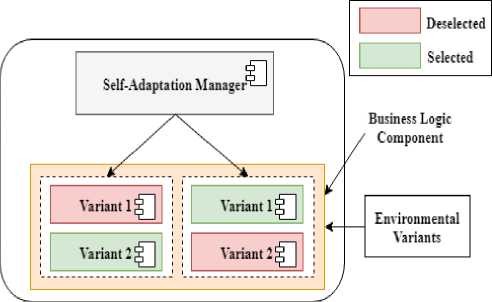
Fig.1. A self-adaptive system.

Self-adaptive systems work in a continuous loop of monitoring, analyzing, constructing plans and executing these. IBM proposed a model named MAPE-K which corresponds to these four processes which are Monitor, Analyze, Plan and Execute with a knowledge base [10]. Monitor process continuously collects information from the system. This information is expressed as metric values such as response time, throughput etc. These are transferred to the Analyze process which detects goal violation. To do this, the Analyze process may compare the metric values with pre-specified thresholds. Goal violation triggers the Plan process which determines the required action sequence for goal conformance. The action sequence can be an alteration of configuration parameter values, substitution of software components etc. In the proposed technique, the action sequence indicates the selection of variants. This plan is realized by the Execute process.

Algorithm 1 Algorithm for Learning-Based Self-Adaptation

Input :   Tm = {Tm,Tm^,Tm3,...,Tm„ } Metric thresholds set dv = {DV1,dv2,dv3 , ,DVn} Variant dependencies set

V e = { V e , V ,,•••, V e } Environmental variants set GTg = {GT G , GTg₂ , GTg₃ , -, GTg_u } Goal types set T _re Regression error threshold

Output:  SV = {SV^, SV, SV,..., SV } Set of software variant selection where SV is 0 or 1

• 1:    Initialize the set of metric equations E_m , utility functions U_m ,

utility values U_v and metric values M_v to 0

• 2:    Generate training data using Algorithm 2

• 3:    if E_m =0 OR Regression error >  T_re then

• 4:              Generate regression model M using training data

• 5:             E_m = metric equations from M

• 6:   end if

• 7:   for i = 1 to n do

• 8:            if GT_g = maximization then

• 9:                      U m,= Em, - Tm,

• 10:              else

• 11:                     Um, = Tm, - Em,

• 12:             end if

• 13:  end for

• 14:   M V = calculate and get current values of metrics

• 15:   U_v = Get utility values by replacing E_m with M V in U m

• 16:    for i = 1 to n do

• 17:              S V = Generate software variant selection using

Algorithm 3

• 18:  end for

As a concrete example of a self-adaptive system, consider a news serving website that provides textual and multimedia-based news to its users. Its architecture is shown in Fig. 2. Multiple servers form a server group which is connected to a load balancer. The goal of this system is to respond within a maximum response time with a minimum content quality. To maintain this response time, multiple servers can be added to the server group. However, server cost must be under a specific threshold. These requirements indicate that a self-adaptive technique should be adopted for this system.

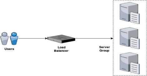
Fig.2. The architecture of a news serving website with load balancer.

Algorithm 2 Algorithm for Knowledge Base Construction

Input : M = { M 1 , M ₂, M 3 ,..., M_n } Metric set

V S = { V S , V S ₂ ,,• - , V S } Software variants set

Output:  Dt = {D^, Dm2, Dm ,..., Dm^} The set of training data for each metric

• 1:    Initialize the training data set D t to 0 and training data size L to

any constant c

• 2:   for i = 1 to n do

• 3:            while L >  0 do

• 4:                          for j = 1 to n do

• 5:                                   Randomly select or deselect V_S

• 6:                        end for

• 7:                         Mv = Get current value of metric M i

• ^8:                           Sv = Get current software variant

selection

• 9:                       D m = D m U{( Sv , Mv )}

• 10:                      L = L - 1

• _11:            end while

• 12:  end for

• 13:   Write D_t to file

• III.    Learning-Based Self-Adaptation with Reusability

The main objective of self-adaptation is to handle goal violations automatically. Goal violation is calculated by observing whether metric values maintain a specific threshold. In this work, goal conformation is calculated using a utility function which is a function of metric values and threshold. Therefore, utility function can be expressed as u_t : m x t ^ R where u_t is the utility function, m is the metric and t is the threshold. The main goal is to find the variant selection that maximizes the total utility of the system. To do this, utility function must be expressed as a function of variant statuses. This is achieved by expressing metric as m : v ^ R, where v is the variant status. A software variant status is 1 if selected and 0 otherwise. An environmental variant status is the value of the related metric. For example, the status of an environmental variant called queue length is the metric value measuring the number of requests waiting in the queue. The relation between metric and variants are constructed by learning from previous data of the form m : v ^ R, which is generated by observing metric values under a random selection of software variants. Best variant selection can be obtained by solving an optimization problem which maximizes the total utility function with respect to the current values of the environmental variants. The learning-based selfadaptation technique is described in details below.

Algorithm 1 shows the proposed learning-based selfadaptation technique. It takes metric thresholds, variant dependencies, environmental variants, goal types and regression error threshold as inputs and provides the best software variant selection. On line 1, the set of metric equation, utility functions, utility values and metric values are initialized as empty. In this paper, we use the variant dependencies mentioned by Esfahani et al. because these are simple equations or inequalities and can be directly fitted into the optimization problem to be constructed [6]. Table 1 shows the variant dependencies which are zero-or-one-of-group, exactly-one-of-group, at-least-one-of-group, zero-or-all-of-group and parent child relation. These are defined as follows.

• 1.   zero-or-one-of-group: This resembles that more

• 2.   exactly-one-of-group : This means that exactly one

• 3.   at-least-one-of-group : This dependency indicates a

• 4.   zero-or-all-of-group : It indicates that either all or

• 5.    parent child relation: This means that enabling a specific variant (parent) requires all other variants of the group to be enabled.

than one feature cannot be enabled.

feature can be enabled at a time in the feature group.

mandatory relationship where at least one of the features in the group must be enabled.

none of the features will be turned on.

Line 2 generates the training data by running simulations using Algorithm 2. It takes metrics and software variants as inputs and provides training data set for each of the metrics. For each metric, each of the software variants is randomly turned on or off (line 5). After all the software variants have been analyzed, the current variant selection is extracted (line 8). On line 9, the current software variant selection and the metric value under that context are added as training data.

Table 1. Variant Dependencies

Variant Type	Variant Constraint	Variant Relation
Optional	n ∑        f n ≤ 1 ∀ fn ∈ zero - or - one - of - group	zero-or-one-of-group
Mandatory	n ∑       f n = 1 ∀ fn ∈ exactly - one - of - group	exactly-one-of-group
Mandatory	n ∑       f n ≥ 1 ∀ f ∈ at - least - one - of - group	at-least-one-of-group
Optional	∑ n       fn mod n = 0? ∀ f ∈ zero-or-all-of-group	zero-or-all-of-group
Depends on Child Features	∀ child ∈ shared features fparent - fchild ≥ 0?	parent child relation

Table 2. Design Pattern for the Components

Component	Subcomponent	Type	Design Pattern
Preprocessing	Preprocessing	Interface	Decorator
	Preprocessing algorithms (e.g., variant selection, normalization etc.)	Class
Learning	Learning	Interface	Strategy
	Learning algorithm (e.g., linear regression, regression tree etc.)	Class
Learning Accuracy Checking	Learning	Component	Observer
	Subject	Interface
	Different notification schemes (e.g., RMSE threshold based, failure count based etc.)	Class
Optimization	Linear Optimization	Interface	Strategy
	Linear optimization algorithms (e.g., Simplex algorithm. Karmarkar's algorithm etc.)	Class
Optimization Problem	Problem Decorator	Interface	Decorator
	Objective Function Decorator	Class
	Variant Constraint Decorator	Class
	Environmental Variant Constraint Decorator	Class

After training data generation, on Line 4 and 5 of Algorithm 1, machine learning algorithm is used to generate metric equations from the training data. In the proposed technique, linear regression is used to generate these equations. This is because linear regression is simple, efficient and produces a linear equation that can be used later to apply linear programming to solve an optimization problem. Linear regression produces the equation similar to (1).

n m. = Vk x v. + c             (1)

i    ii i=1

Here, m denotes the metric, v is the variant, and k and c are the slope and intercept respectively. Metric equations are reconstructed if the regression error (e.g., RMSE) is greater than a specific threshold (line 3).

Algorithm 3 Algorithm for Software Variant Selection Input :  Uv Utility value of the ith metric dv = {DV1,dv2,dv3 „ Dvn} Variant dependencies set

V_e = { V e , V e₂ ,,•••, V ? } Environmental variants set

U m = ^{{ U}m ,, U m 2, U m, , • • •, U m n ^{} Utilit}y functions set E m = ^{ E m ,, E m - E m, ,■",^Em„ ^} Metric equations set

Output: S V = { S _V^ , S V , S V ,..., S V } Set of software variant selection where S_V is 0 or 1

• 1:    Initialize the maximization objective function F to U , the

max     mi set of optimization problem OP and environmental variant constraints Ce to 0

• 2:   if U_v <  0 then

• 3:             V s = Get software variants from E_m

• 4:             for j = 1 to n do

• 5:                      V s = Get software variants from E_m

• _6:                    if V S CI V S *0 then

F =F

• 7:                                      max ¹ max ^{+ r} Sj

• 8:                      end if

• 9:             end for

• 10:            for j = 1 to n do

• 11:                      E_e = Get current value of V_e

• 12:                     C e, = C e, U(" V e = E e ")

• 13:           end for

• 14:         OP = OP U F maxU DV U C

v

• 15:            S V = Solve OP using Linear Programming

• 16:  end if

These metric equations are used to generate the utility functions (line 7-13). The metric thresholds and goal types are further required for this purpose. This work defines two goal types based on the type of optimization problem namely maximization and minimization. For maximization goals, where the metric values need to be more than the provided threshold, the generated equation has the form similar to (2).

UtUity_n = Metric_n - hbrehOodd _n        (2)

Here Utility is the utility value, Metric is the metric value and Threshold represents the metric threshold value for the n^th metric. The utility function for minimization goal can be constructed similarly.

These utility values are continuously monitored for goal violation. From (2), goal violation occurs if utility value is less than zero. The goal violation and the software variant selection procedure are shown in Algorithm 3. In case of goal violation (line 2), the optimization problem is constructed. The goal is to maximize the total utility function value of the violated goals. These goals are related because two metric equations may have overlapping variants which makes these metrics dependent. Hence, the violated utility function may have dependencies with other utility functions indicated by the shared variants in their corresponding metric equations. The summation of all these dependent utilities constructs the maximization objective function. On line 3 to 9 in Algorithm 3, the construction process of this function is shown. Furthermore, the current values of the environmental variants are extracted and added as constraints from line 10 to 13. On line 14, the linear optimization problem is constructed using the maximization function, variant dependencies and environmental variant constraints. This linear optimization problem is solved to get a software variant selection (line 15). This software variant selection is the final output of the algorithm that is used to turn on or off software variants. Thus, the most optimal feature selection subject to the variant dependencies and current environmental status is executed.

The components of the self-adaptation manager have been organized with Gang of Four (GoF) design patterns so that these can be reused and customized easily [11]. These are selected by matching the intent of the design pattern with the intent of the components. Table 1 shows the components, subcomponents and the design patterns. These design patterns and their applications in the proposed approach are discussed below. A detailed discussion of the GoF design patterns is out of the scope of this paper. Interested readers are referred to [11].

• •    Strategy Pattern: Strategy pattern is used when algorithms need to be varied independently. Adding an algorithm involves only implementing the abstraction and passing its reference to the invoker of the algorithm. Thus, it promotes customizability and reuse. This is why this pattern has been used to support reuse and customization of the learning algorithm and linear optimization algorithm (Table 1).

• •    Decorator Pattern: Decorator pattern is used when functionalities need to be added dynamically. Decorator pattern has been used for the preprocessing logic (Table 1). If two preprocessing algorithms such as normalization and feature selection are used, this pattern helps to

pass the normalized data to the variant selection component and forward the selected features to the learning algorithm. Decorator pattern helps to add any object within the flow easily. For example, if anyone wants to add missing data handling, he needs to create a class and insert it between normalization and variant selection which involves changing only two references. For the same reasons, the decorator pattern has been used to add attributes to the optimization problem when adaptation is required (Table 1). The variant constraints, environmental variant constraints and the objective function are added to build a complete optimization problem. Then, it is passed to an optimization algorithm for receiving an optimal variant selection. As the problem is built at runtime gradually, Decorator pattern is suitable for this purpose.

• • Observer Pattern: This is used when a notification scheme is needed. For this, it has been used to notify the learning process to start again because a new pattern has arrived (Table 1). To achieve this, the learning component has to act as an observer that registers to a subject that sends notifications. For example, RMSE threshold based subject will notify the learning component when the RMSE will be higher than a specific threshold.

Applying design patterns for self-adaptive system design helps to maintain a consistent structure of the adaptation manager. For this reason, modifying and reusing any part of it becomes easier. The proposed methodology incorporates design patterns as a part of the adaptation component design mechanism to ensure that systematic reuse can be achieved.

• IV. Experimental Setup

The proposed technique was tested on Znn.com which is a model problem by Cheng et al. in the repository of the Software Engineering for Self-Adaptive Systems community [12]. The Znn.com system has been used in numerous papers for evaluating their adaptation approaches [13, 14, 15, 16, 17]. This is why Znn.com has been used to assess the proposed methodology.

Znn.com is a news serving application similar to Fig. 2 which provides textual and multimedia-based news to its users. According to the Znn.com specification, it follows an N-tier style where a load balancer is connected to a server group. The clients send their request to the load balancer and it distributes the requests among the servers in the server group. The business goals of Znn.com are related to performance, content fidelity or quality and server cost. The main goal is to provide service with a minimum content fidelity and within the budget while maintaining a minimum performance. These goals are related to one another. For example, if content fidelity gets higher, server performance will decrease because the response size is larger due to better content quality (e.g. high-resolution images). Hence, a new server needs to be added from the server group. However, servers cannot be added infinitely because the total cost of all the added servers must fall within a specific range. All these scenarios make the satisfaction of multiple goals a nontrivial task. Therefore, Znn.com requires a self-adaptive mechanism to optimally work under multiple goals.

Another scenario where Znn.com demands adaptation is when the news website is under a high load situation, known as the Slashdot Effect. As mentioned by Cheng et al. in [13], if a website is featured in slashdot.org [18], it gets crowded with visitors within a few hours or days. Due to hit from multiple users, the website might be temporarily down. To partially solve the scenario, some applications such as Gmail request the users to reload later when such a high load situation is detected. However, this is not expected because it hampers the service level of the application. For this reason, a selfadaptation scheme is required which repairs the system and brings it closer to the three goals mentioned in the previous paragraphs.

Znn.com was deployed on five virtual machines which were connected to another virtual machine acting as a load balancer. Two more virtual machines were used where one helped to collect metric information and the other one helped to simulate user requests. Each of the virtual machines had the following configuration.

• •    Operating System: Ubuntu 14.04 LTS

• •   RAM: 512 MB

• •    CPU: 3.30GHz Intel Core i3 Processor

• •    Platform: 32 bit

• •   Virtual Disk: SATA Controller 8 GB

The implementation of Znn.com was done with PHP and MySQL. The effectors were written in Bash scripting language. In each of the server machines, apache2 web server was used to deploy Znn.com. Apache JMeter was used to simulate user requests in the user requests simulation environment. In the metric collection environment, PHP codes were deployed using apache2 web server which was used to calculate the metric values of performance, cost, content fidelity and the environmental variants.

Before starting the experiment, the variants and variant dependencies of Znn.com were specified. As software variants are entities that can vary and can be toggled (turned on or off), it is evident that every server is a software variant. This is because adding a server means turning it on and removing means otherwise. Cheng et al. mentioned that content fidelity has three types which are high, low and text [13]. Each of these is a software variant which can be toggled. The server variants belong to the at-least-one-of dependency group. This is because at least one of the servers must be turned on to serve contents. Moreover, exactly one of the content fidelity variants can be selected and so, these belong to the exactly-one-of variant dependency group.

After choosing variants and variant dependencies, metrics and utilities were chosen. Response time, content size and number of active servers were used to calculate performance, content fidelity and cost respectively. The thresholds for each of these which are maximum response time limit, minimum content fidelity and maximum number of active servers respectively, were chosen. As the operating environment of software is vastly dynamic, these thresholds are likely to vary in different systems. For environmental variants, service time and request arrival rate were chosen.

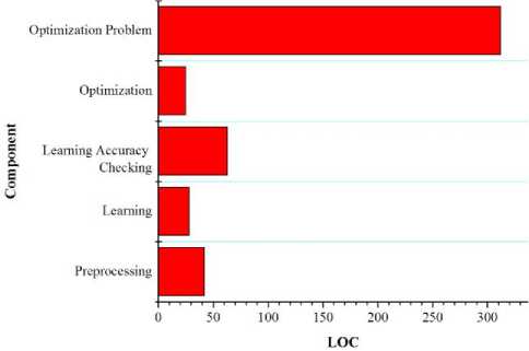
Fig.3. LOC Distribution of Components.

In order to access effectiveness, the system was put under a situation representing the Slashdot effect. To do this, the experiments provided in [7] were repeated. However, each of the experiments was tuned down to around 15 minutes and load five times higher than the mentioned experiment was provided which is mentioned below.

• •    15 seconds of load with 30 visits/min

• •    2.5 minutes of ramping up to 3000 visits/min

• •    4.5 minutes of fixed load to 3000 visits/min

• •    9 minutes of ramping down to 60 visits/min

The situation was simulated using the Throughput Shaping Timer plugin of Apache JMeter1. The Gaussian Random Timer of JMeter was also used to provide short delay within requests to represent real-life behavior.

Table 3. Descriptive Statistics for LCOM4 and MPC of the Proposed Method

Metric	Minimum Value	Maximum Value	µ	σ
LCOM4	0	3	0.8923	0.75256
MPC	0	17	3.046	4.40678

For assessing reusability of the proposed approach, three metrics were used which are Lines of Code (LOC), Message Passing Coupling (MPC) [8] and Lack of Cohesion of Methods 4 (LCOM4) [9]. LOC was used in the Rainbow framework by Cheng et al. for assessing reusability [7]. However, LOC, as a measure of reusability has been criticized in some of the literature because LOC does not represent the connections between and within the classes or modules [13, 19]. This is why coupling and cohesion based metrics were used. It has been seen that reusability depends on coupling and cohesion of classes as low coupling and high cohesion increases the chance of reuse [20]. For this reason, MPC and LCOM4 were used to measure the reusability of the approach. These metrics are described below.

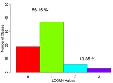
Fig.4. LCOM4 Distribution of Components.

О 1   2   3   4   5   6   8 10 11 12 13 14 17

MFC Values

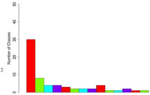
Fig.5. MPC Distribution of Components.

• •    LOC: LOC counts the number of lines in the code. However, issues such as, whether comments, blank lines etc. will be considered are a concern. David Wheeler developed a code analysis tool named SLOCCount ² , which was also used by Rainbow for counting LOC. In this tool, a LOC is considered as a line terminated with a newline, which contains at least one character excluding whitespaces and comments. To validate the proposed methodology, SLOCCount was utilized to calculate LOC. The lower the LOC, the higher the probability of reuse.

• •    MPC: According to Fenton et al., MPC is a valid measure of coupling and so, a valid measure of

  1

  
  

reusability [19]. MPC indicates the number of external invocation of methods from a class. For example, if a class calls 5 methods of some other classes, the value of MPC for this class is 5. MPC was used to measure the coupling between the classes of the adaptation manager after it was integrated with Znn.com. The higher the MPC, the higher the class is dependent on other classes, therefore, the lower the reusability

• •    LCOM4: LCOM4 is a measure of cohesion. Cohesion indicates the strength of internal relationships of functionalities within a class. LCOM4 is the number of “connected components” within a class [21]. A connected component consists of a group of methods which either call one another or share at least one instance variable of the class. The presence of multiple connected components for a class means that the class performs multiple unrelated responsibilities. Hence, cohesion and reusability increase as LCOM4 decrease. The ideal values of LCOM4 are either 0 or 1 [21].

To assess the effectiveness of adaptation, the experiment was performed five times starting from a single server and high fidelity variant selection. This is because this feature selection results in the worst performance. Every time one of the five servers was chosen and the load was increased by any constant factor. In the experiments conducted, the load was increased by 120 visits/min and it was observed that the system reaches its maximum capacity after five runs. In each of the runs, it was observed whether the proposed methodology could gradually improve performance. Following the literature, the value of the main objective response time was compared in two situations, namely adaptation and without adaptation [3, 6, 13].

• V.    Result Analysis and Discussion

  Fig. 3 shows the LOC distribution of different components. It is evident that the first four components have relatively lower LOC. However, the Optimization problem component has a higher LOC because it consists of a higher number of classes. Upon further investigation, we observed that the average LOC of this component is 35 which is close to the average LOC of the other components. Therefore, the classes are short and stable in size indicating better modularity and better reuse. Table 3 shows the minimum value, maximum value, mean and standard deviation of LCOM4 and MPC. For LCOM4, the highest value is 3 and the lowest value is 0. The mean and standard deviation of this metric is 0.8923 and 0.75256 which indicates that LCOM4 values are close to the ideal values (0 and 1). The mean and standard deviation for MPC is 3.046 and 4.40678 which shows

that MPC values are low on average. This indicates low coupling between classes.

These results are more clearly visible from Fig. 4 and 5. From Fig. 4, it is seen that 86.15% classes have LCOM4 values of either 0 or 1, where 13.85% classes have values different from these. Therefore, 86.15% classes have achieved maximum cohesion. Fig. 5 shows the number of classes for each of the MPC values. It is evident from the figure that most of the classes have low MPC values. This shows that the proposed methodology results in loosely coupled classes. Hence, according to the discussion in Section II, low coupling and high cohesion show the reusability of the proposed technique.

The five runs of the adaptation logic for Znn.com is depicted in Fig. 6. It is visible from all the five figures that adaptation gradually improves the performance of the system. The threshold chosen for performance was 6.2 milliseconds (ms). From Fig. 6(a), it is seen that response time instantly decreases after approximately 10 requests and increases after approximately 18 requests. After this, the response time stays constant because of the fixed load of 3000 visits/min as mentioned in Section II. Overall, the proposed adaptation technique helps to quickly decrease the response time down to 6.2 ms and remain there. The response time threshold is frequently exceeded for the technique without adaptation.

A similar pattern is seen in Fig. 6(b). The adaptation mechanism reduces the response time from the large spike after approximately 15 requests down to almost 5 ms. The system performs worse overall without adaptation because the response time is higher than the threshold from 12 to 38 requests approximately.

From Fig. 6(c), the response time line also decreases after 15 requests. The response time becomes less than the threshold after approximately 15 requests and remains unchanged up to approximately 35th request when a violation of the response time goal is observed. However, under the proposed adaptation technique, the response time quickly drops back under the threshold and stays there throughout the run.

Fig. 6(d) shows a similar pattern like Fig. 6(c). However, considering the aforementioned four figures, it is clear that adaptation quality is gradually improved because the average distance between the adaptation and without adaptation lines becomes distant. This happens due to the continuous update of the knowledge base and training which ensures that the prediction model is up-to-date throughout the time.

Fig. 6(e) represents the run with maximum load. Here, the response time varies unstably. However, the adaptation mechanism still shows better performance than the system without any adaptation. Throughout the run, the mechanism without adaptation goes above the threshold where the system with adaptation violates the response time goal only five times, however, immediately reduces down to the threshold limit.

With Adaptation

Without Adaptation

With Adaptation

Without Adaptation

(a) Run 1.

With Adaptation

Without Adaptation

Requests

(b) Run 2.

Requests

(c) Run 3.

(d) Run 4.

(e) Run 5.

Fig.6. Comparison of Performance: Adaptation vs Without Adaptation in Five Runs

Requests

Requests

With Adaptation

Without Adaptation

With Adaptation

Without Adaptation

• VI.    Related Work

Architecture-based self-adaptive systems operate on architectural models to detect goal violation and perform actions on the managed system through the model. Rainbow framework is a seminal architecture-based selfadaptation approach which achieved reusability of the overall infrastructure [7, 13]. However, the system components were not reusable and the strategies were hard-wired static ones. MADAM framework proposed by Flock et al. used predefined utility functions to select the highest utility reconfiguration of the model [22]. Although their model was more dynamic, the reusability of the self-adaptation was not addressed and the utility functions were required to be predefined. Gui et al. proposed the Transformer framework where strategies of a specific goal were composed in a module which they termed as Composable Adaptation Planner (CAP) [23]. As it was based on static strategies, problems similar to the Rainbow framework were present.

Another dimension towards designing self-adaptive systems is based on control theory. One of the earliest approaches is the hierarchical model-based autonomic control proposed by Litoiu et al. [24]. The managed system was attached to three levels of controllers or selfadaptation managers namely component, application and provisioning controller. The component controller maintained a model of a component which was tightly coupled to the controller. Therefore, the reusability level of the controller was low. Müller et al. proposed a high-level design for a feedback-control driven self-adaptive system [25]. As it was mentioned that the controller code and core system code could be intermingled, the reusability level was low.

Several techniques based on component models have been proposed. Examples of these techniques include the K-Component framework by Dowling et al. [26], Fractal component model based framework by David et al. [27], and Fractal and dynamic Aspect Oriented Programming based approach by Wu et al. [28]. Although the component model based techniques achieved high reusability within the same component model, reuse between component models was difficult. Current selfadaptation techniques are mostly based on machine learning due to the aforementioned reasons. Reinforcement learning based techniques such as model-free Q-learning based technique by Kim et al. [3] and self-adaptation using model-based reinforcement learning by Ho et al. [4] were proposed. Nevertheless, these techniques are prone to state space explosion for large-scale systems. Moreover, the issue of reusability was not addressed. Esfahani et al. proposed the FUSION framework which determined an application feature (variant) selection by solving an optimization problem that maximizes total system utility [5, 6]. Similar to our proposed approach, they expressed metrics as a function of features to derive utility functions. However, they ignored the environmental variants which are essential for an effective adaptation. Additionally, FUSION did not explicitly address the issue of reusability.

In this paper, two types of variants are used namely application and environmental variants. In the optimization problem, the current values of the environmental variants are used. Hence, all the application variant selections are specific to a particular environmental instance. This leads to better selfadaptation. The adaptation approaches in the literature lack such a unified approach of application and environmental variants. Moreover, although some techniques discuss reusability of the whole selfadaptation manager, none of these address the reusability of the components of the manager. The proposed technique addresses this issue by designing the selfadaptation manager components using design patterns.

• VII.    Conclusion

Reducing the effort of manual maintenance of software is the core objective of self-adaptation. The reusability of self-adaptation managers can further reduce the effort of building a self-adaptation solution. The proposed technique is aimed towards proposing a solution to selfadaptation that is both effective and reusable at the component level. This is achieved by incorporating environmental variants with software variants and using these to form an optimization problem for maximizing the total utility of the system. The total utility is constructed using the utility functions of violated goals. These utility functions are expressed using metrics and their thresholds which are further expressed in a linear form applying linear regression learning algorithm. This linear form helps to state metric as a function of variants, both software and environmental. In the optimization problem, the environmental variants and their current values are used to generate constraints. The solution to this optimization problem is a software variant selection under the current values of the environmental variants. During the design of the self-adaptation manager, design patterns have been used to ensure reusability. In the paper, these design patterns are described which have been selected by comparing their intents with the intents of self-adaptation manager components.

The approach has been validated using a news serving website named Znn.com. Low values of LOC, MPC and LCOM4 showed the reuse potential of the self-adaptation manager components. The response time of the website was observed under with and without adaptation. It was seen that the proposed self-adaptation technique stably improved response time. Conversely, the response time varies rapidly when adaptation is not applied.

Acknowledgment

This research has been partially supported by The University Grant Commission, Bangladesh under the Dhaka University Teachers Research Grant. Reference No: Regi/Admin-3/2017-2018/68450-52.