An Evaluation and Improved Matching Cost of Stereo Matching Method

Published Online October 2016 in MECS

The recent flow in the popularity of 3D films offers a particular opportunity for 3DTV. The main key to development of 3D display technologies is depth perception; it can be provided to show as an amazing place. Stereo vision algorithms are reconstructed 3D scenes through matching multiple images taken from slightly different viewpoints. The important task in machine vision field is defining of 3D data from images. Stereo matching algorithms are important to decide correspondences between the two views [1] [2].

There are a number of algorithms which have been implemented for depth and disparity maps [11]. Stereo matching algorithm can be divided into two categories; (a) local methods (b) global methods. Local method can be classified into two categories as well (a) area based algorithm (b) feature-based algorithm. Area-based algorithms use Normalised Cross Correlation (NCC), Sum of Absolute Differences (SAD) and Sum of Squared Differences (SSD). Window based technique is an example of area based method. Feature-based algorithms match edge corner as the extraction of feature from images and it is fast but they generate light disparity or depth maps. Global method energy minimization function is defined as the combination of data and smoothness energy. These methods have high computational complexity and are very expensive. Dynamic programming is the example of global methods [7] [12].

• A. Related work

Mukherjee et al. [2] proposed a region and block based stereo matching algorithm. K-Means clustering segmentation is used for removing a lot of redundant boundary pixels. It is determined the boundaries disparities by SAD algorithm. Next step is segmentation using morphological operations and SAD algorithm to remove the redundant boundary pixels. At the end results are reconstructed using disparity map.

A frame work divides the color images into different regions and applies various methods customized to each region. Different region segments the Low Resolution (LR) depth map for smoothening [4]. Multiple image segmentations obtained by different super-pixel generation method. Color image divides continuous and discontinuous regions. In continuous region, LR depth is interpolated to High Resolution (HR) without color information. In discontinuous region HR depth value obtain by histogram method. This method improves both qualitative and quantitative depth map up sampling.

Hu et al. [5] proposed novel algorithm for evaluation of 17 confidence measures for stereo matching comparisons.

Area based stereo matching algorithm is used for real time system to generate disparity maps. The proposed algorithm computes the disparity map using two correlation windows (a) large sizes (b) small sizes. SAD algorithm is used to find initial disparity map and left right consistency check to detect unreliable pixels. Disparity interpolation is used to assign new disparity values for reliable neighboring pixels. Using a reliable pixel and intensity of an unreliable pixel computes the distance between the two dissimilar pixels. Disparity refinement remove outline of color segment and increases accuracy of the algorithm [8]. Section II describes the proposed stereo matching algorithm. Section III shows the performance parameter to be used for check capability of the algorithm. Section IV shows the results of depth estimation and measure the quality of results. We conclude the paper in section V.

• II.    Proposed Work

Stereo matching methods basically done by four steps: matching cost calculation, cost aggregation, disparity calculation, and disparity refinement. Here three frames were applied for generation of depth map. First frame is preprocessing using color space conversion rgb2lab and rgb2xyz conversion. Specification, visualization and creation of the images are defined by color space method. Second frame is stereo matching method to find initial matching cost for each pixel at all possible disparity level cost are aggregated with minimum error. Hole filling, permutation of morphological operator and median filter technique are applied at post-processing (third frame) to obtain noise less, reliable, smooth and efficient depth map.

• A.    Preprocessing

The different color space present that makes certain calculations more suitable and provides a way to recognize colors that is more perceptive. Most imaging equipments store captured images in the RGB format which models the output of physical devices but does not properly visualize. The lab color space was developed to aspire for uniformity in human eye. Human eye is more sensitive to changes in brightness than color. The “L” component of the lab color space closely matches for the easy human perception. There are many image processing algorithms applying the important transformations discussed in [1] [9]; we convert the left and right images from RGB to the Lab color space and retain only the L values of its pixels for further processing. The color space xyz conversion is also used for result comparison with the lab color space. The color space rgb2xyz is defined only positive values and Y is luminance.

• B.    Stereo matching

We used block based horizontal pixel matching technique and zero depth assignment process. In order to construct raw depth matrix for every disparity can be expressed by,

• 1    i + r j + c   3                                    2

d ( s , t , Hsm ) = — X X X ( IL ( s , t , k ) - IR ( s , t - Hsm , k )) 3 ' r ' c s = i t = j k = 1

where H sm =Maximum shifting at horizontal; k=R, G, B component take value 1, 2, 3 respectively; r, c= number of row and column respectively.

For a set horizontal shift value measures how different is pixel corresponding to the point t in the left image compared with the pixel matched with right image. Guided filter is filtering method between image and a second guidance image. The guidance image can be the image itself, a different version of the image, or a completely different image. Guided filter is a neighborhood operation; it calculates the output value of pixels statistics of a region in the corresponding spatial neighborhood in the guidance image [14]. It is used to reduce sharp transitions, de-noising and incorrect matching in images. N x M window size guided filtering is applied to d(s, t, Hsm).

Guided filter is the fast edge-preserving non approximate linear time filters. It is effective and efficient in a great variety of computer vision, computer graphics, edge-aware smoothing, detail enhancement, compression, image matting and feathering etc. The guided filter output ᶃƒo at a pixel i is mathematically expressed as a weighted average in (2).

ᶃƒ = ∑    ( )                 (2)

Where i, j are pixel indexes. The filter kernel Wij is a function of the guidance image I and independent of p. This filter is linear with respect to p [14]. By applying guided filter, Wij filter kernel can be expressed by (3),

(       )(       )

_, = _{| |} ∑ _{:( , ) ∈}   (1+              ))          (3)

Where, , are the mean and variance of wk in I. is a smooth parameter, |  | is the number of pixels in window with fixed dimension.

For proper horizontal shift value, the minimum value is start from 0. The maximum horizontal shift (H sm ) value is the maximum value of the pixel in the ground truth map, divided by the scale factor as expressed in (4).

Hsm=                     (4)

Where, H sm – Specified Range of the object, b is the baseline means distance between the centers of the cameras, f is the focal length of sensor, x is the pixel size, N maximum disparity value. The window is only shifted along the x direction define as H_sm. To compute the difference, a window is placed fixed at left images, while Hsm is shift over finite range in the right image.

Further guided filtering output applies minimum difference value assignment function with minimum error for each disparity. The minimum error energy g (s, t, Hsm) is the reliable depth estimation for pixel (i, j) of raw depth map as mathematically expressed in (5).

ᴆ r (s, t) = min {g(s, t, H sm )}              (5)

Algorithm 1 and 2 show the mathematical process code of the depth map method.

Measurements are the measure area, length, curvature of an object. It reduce the pixel configuration of an object to a single scalar number, such measures will hide much of the detailed shape information of the original object. Therefore many applications can be handled well using only global scalar shape measurements. The area of an object can be determined by counting all the pixels contained in the object. The perimeter is the total length of the object boundary. The object boundary is the collection of all boundary pixels, which are all object pixels that have a non-object pixel for a neighbor.

Algorithm 1 Guided stereo matching

Ĭ Cr , Ĭ Cl – color space conversion right, left output

Ϛ – color component r, g, b

Ħ S , Ħ SM - horizontal shifting, maximum shifting at horizontal

Ͼ L – cost limit, ₽ u, ₽ d - Perimeter up, down

ᶃ ƒ , ᶃ ƒo – guided filter and output

ᴆ r , ᴆ am , ᴆ ao, ᴆ f – raw depth, minimum depth assignment, depth assignment output, final depth

₽, ₽ O – perimeter

₥ f – median filter

Ș MC – stereo matching cost output

Ӈ f , Ӈ fo - holes filling, output

₽ M , ₽ MO - permutation of morphological operation-

(Đ, ɛ, ʗ, ȍ - dilation, erosion, closing, opening) and output for ĦS = 0 to ĦSM for ĦS to column for 0 to row

ȘMC = ȘMC + [ ĬCl(s,t, Ϛ) - ĬCr(s, t- ĦS, Ϛ) ]2 end end

ᶃ ƒo = ᶃ ƒ (Ș MC )

for s = 1 to row for t = 1 to column if ϾL > ᶃƒo

ᴆr= ᶃƒo end end end end end

₽ O = ₽( ᴆ r )

ᴆ ao = ᴆ am (₽ O ) (See algorithm 2)

Ӈ fo = Ӈ f (ᴆ ao )

₽ MO ⁼ ₽ M (Ӈ fo )

ᴆ f = ₥ f (₽ MO )

The perimeter can be measured by tracing the boundary of the object and summing all the steps of length. The perimeter will generally increase with increasing resolution, while the area will converge to a stable value. A pixel is part of the perimeter if it is nonzero and it is connected to at least one zero-valued pixel see in fig. 3 step number 5.

For zero depth map assignment we count the disparity map whose disparity is not defined. For that we create a map in which the disparity is calculated by its neighbor pixel in the same column which lies above the said reference pixel. Similarly, we create another map to compute disparity of said pixel in downward direction along the same column. After this process we get two different disparity maps among one in above direction and one along the downward direction.

Finally we compute the finishing disparity map which compares the prior two different disparities which we earlier obtained.

Algorithm 2 Zero depth assignment count = 0

for 1 to column for 1 to row if ₽O = 0

₽u = count else count = row end end end for 1 to column for 1 to row if ₽O = 0

₽d = count else count = raw end end end for 0 to row for ĦSM to column if ᴆr = 0

ᴆao = min ((ᴆr (₽u), column), (ᴆr (₽d), column)) end end end

• C.    Postprocessing

Filling stage is the key part of our method and completed the final result. Mathematical morphology operation is used as a tool to extract image components. These are useful in the description and representation of region shapes. Region filling operation is based on a set of dilations; complementation and intersections to fill the holes in the grayscale image. ‘I’ is the region or more connected components. We form an array X_k the same size as the array containing ‘I’ whose elements are zeros (background values), except at each location known to correspond to a point in each connected component in I, which we set to one (foreground value). The purpose is to start with X 0 and find all the connected components by the iterative procedure expressed in (6).

X k = (X k-1 Ф B) n I c , k= 1, 2, 3... (6)

Where B is structuring element, the procedure terminates when X_k = X_k-1 with X_k containing all the connected components of I .

The permutation of morphological operators are dilation, erosion, opening and closing operation with structuring element neighborhood with specific matrix 0’s and 1’s. Morphological operator a dilation operation enlarges a region, while erosion reduces the size. A closing operation can close up internal holes in a region and smooth the contours of image. An opening operator removes the regions of an image that can’t contain structuring element. The mathematical morphological operator is expressed in (7), (8), (9), (10).

D (j, k) = P (j, k) Ф Q (j, k) = {z/(gz)nA*0}(7)

E (j, k) = P (j, k) 0 Q (j, k) = {z/(B)zCA}(8)

O (j, k) = P (j, k) o Q (j, k)

= {(P (j, k) Θ Q (j, k)) ⊕ Q (j, k)}(9)

C (j, k) = P (j, k) • Q (j, k)

= {(P (j, k) ⊕ Q (j, k)) Θ Q (j, k)}(10)

Where, P (j, k) = Image, Q (j, k) = Neighborhood element, D, E, O, C = Dilation, Erosion, Opening and closing operation respectively.

The different size and shape of structuring elements are rectangle, box, circular, disk and random. The function of the structuring elements is interacting with image. Central pixel of a symmetric structuring element may be denoted as its origin or any. Through reference point, translate the structuring element can be placed anywhere on the image. It can be applied to the image for enlarge or reduce a region, shape etc. Morphological opening operation remove thin protrusions, smooth object, break thin bond and removes regions cannot control the structuring element. Morphological closing operation smooth objects same as opening operator. Closing operator join the narrow breaks, fill hole smaller than structuring element and fill long thin gulf. In structuring element if we put number of 1’s in right side with dilation operation, the object’s region is enlarged, whereas in erosion same operation reduce the object boundary. In our algorithm we are using random structure [1 1 0; 0 1 0; 0 0 1] and [1 1; 0 0] etc. Non linear spatial filter also called rank filter is performed to reduce the noise and this improves the output of the depth as a grayscale image is applied at the end of the stage.

• III.    Parameter For Quality Assessment

We evaluated the performance of proposed stereo matching algorithm with JBU, WMF, SAD, SHD and SSD methods [6] [10] [15] [16]. The results of the proposed algorithms are evaluated with Structural Similarity Index Map (SSIM) and Peak Signal to Noise Ratio (PSNR).

SSIM index is a reference metric measuring image quality based on ground truth. The SSIM index measures the similarity between two images. It computes three terms (a) luminance term (b) contrast term (c) structural term expressed by (11).

SSIM(s , t) = [l(j, k^“ [c(j, k]^ [s(j, kW(11)

Where,

I (j ,k) =

(i f ⁺ il + ^c i )

c (j ,k =

-C^W+j^ ⁽of ⁺ ^k ^{+ C} 2 )

(Oj+ c)) s (,k = 7

(O j O k + c₃)

Where, μ x , μ y , σ x , σ y , σ xy and c are the local means cross-covariance, standard deviations and constant for images. If α = β = γ = 1, C3 = C2/2 the index is expressed by (12).

SSIM (j , k) = ^^(JZi'L^L    (12)

(m J + M к +C l )( O j + ct J + C ) )

PSNR measure the quality measurement between the ground truth and a resultant image expressed by (13).

p2

PSNR(k, ) = (rn* n)10lo_{S1 0}                  (13)

Where M and N are the number of rows and columns respectively; “R” is the number of image gray levels. PSNR calculates the peak signal to noise ratio in decibels (dB) between ground truth and resultant images. The higher the PSNR, the enhanced the qualities of the disparity map [17].

• IV.    Results And Discussion

Fig. 1 shows the Middlebury dataset, ground truth images, depth map and SSIM map [13]. Fig. 2 and 3 shows the mathematical output of experiment image variable in MatLab workspace. There are total 8 steps which show the resultant numerical value of image. Step 1 is the preprocessing step in which the rgb2lab and rgb2xyz color conversion function is applied for suitable mathematical calculation. It is mandatory to apply padding to cover boundary pixels in a particular operation. Basic block matching function is applied to the next step number 2. The output of block method is not accurately differentiated between two images. There are number of pixel which are not assigned to its proper value and remain null. Therefore the combination of block method and guided filter function perform robust matching. Guided filter is divided into different window size (N x N) like 3, 5, 7 and 9 in step number 3. The step number 4 is the process with the guided filter and block matching to assign the minimum difference between stereo pair.

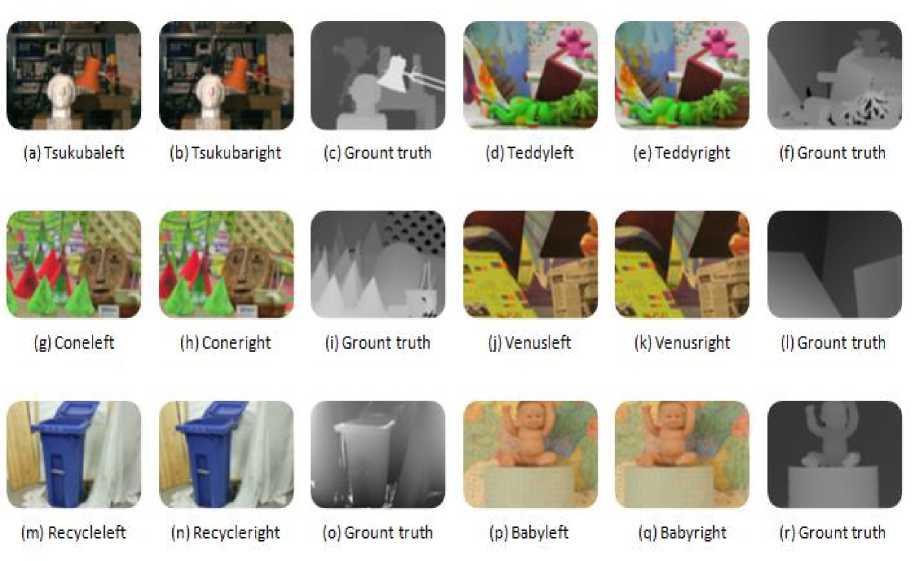
Fig.1 Middlebury stereo dataset with ground truth images [13]

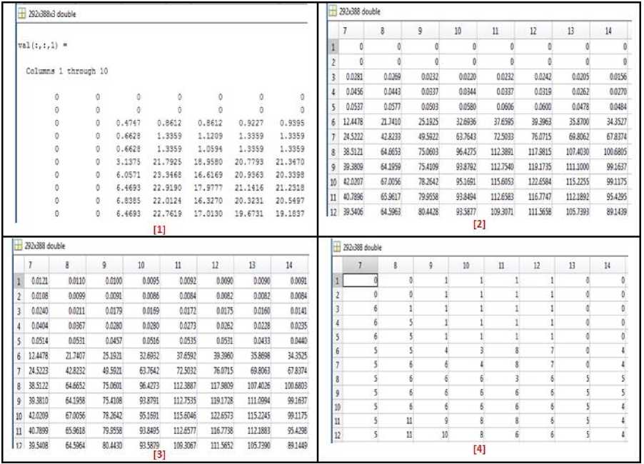
Fig.2 Numerical output of MatLab workspace variable for our algorithm

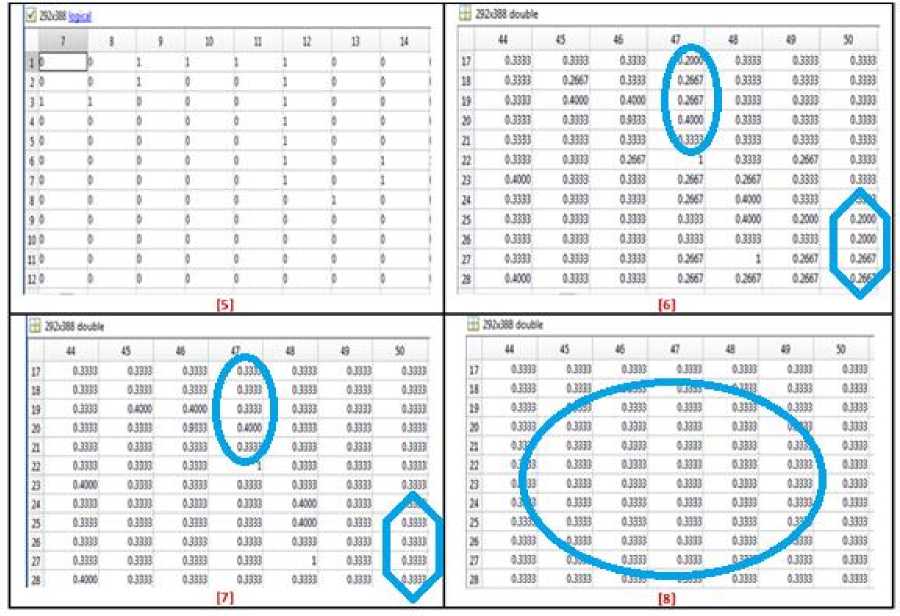
Fig.3. Numerical output of MatLab workspace variable for our algorithm

The perimeter mathematical process is the next step to tracing the boundary of the object and summing all the steps of length. In this map some pixels have not assigned value yet so next step is to assign the value. With the help of perimeter function assign value embed at zero value in the map. Here dissimilar pixels are set to unknown shown in fig. 3 step number 5 and 6. Next step number 7; these pixels are filled using hole filling operation. Morphological operation like filling function used to fill the small gap and unknown pixel of the gray scale results. Next we apply the permutation of morphological function operators are dilation, erosion, opening and closing operation with structuring element neighborhood with specific matrix 0’s and 1’s. Depth maps are generated using 3, 5, 7 and 9 neighborhood size (N x N) of median filter at the end of the stage shows the results in table 1 to 3. Median filter reduces the noise and black specks around the border. The effectiveness in results is shown in fig. 3 enlarge with oval and hexagon.

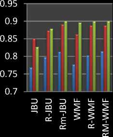
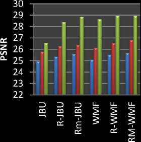
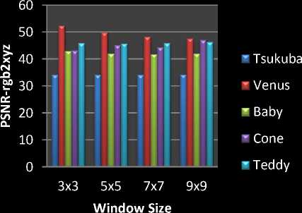
The results of our algorithm are presented in table 1 to 4 and Fig. 6 and 7. Tables I, II and III, IV show the PSNR and SSIM of our algorithm tested on standard Middlebury images like Tskuba, Baby, Teddy, Cone, and Venus images [13]. Fig. 4 shows the performance of PSNR and SSIM of algorithm JBU, R-JBU, RM-JBU, WMF, R-WMF, and RM-WMF [10]. Fig. 4 and 5 show statistical features of PSNR and SSIM. The comparison of image quality for PSNR shows that for image where the depth structures are maintained, the quality is improving as shown in table I, II and IV as compare the other algorithm [10]. SSIM of proposed method is also improving the already existing algorithm shown the statistical features fig. 4 and 5.

Table I and II shows the PSNR and SSIM of Tsukuba and Venus image. We applied Hsm 15, 20, 25 and 30. The quality of PSNR and SSIM at the 20 shifting point is optimum and best matching pixel. The quality of PSNR and SSIM is increased in rgbtolab conversion compare with rgbtoxyz conversion in tsukuba images. Window size increases the PSNR and SSIM also increases.

Table III shows the SSIM baby, Cone, Teddy and recycle images. Here Hsm 45, 50, 55 and 60 because the best matching is done in this shifting points. The quality of SSIM at the point of 60 H sm is optimum and after it is reducing. So the best matching map is at the value of 60

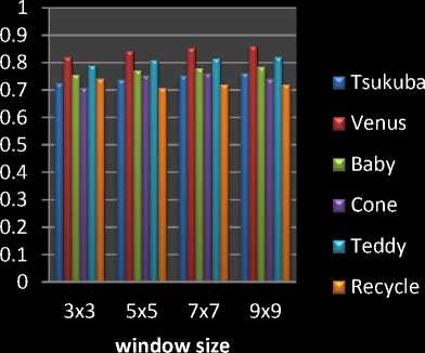
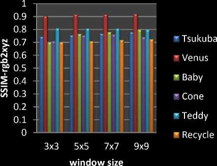
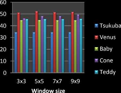
Fig. 4 and 5 shows the comparative analysis graph of SSIM and PSNR with different window size.

Table I. Performance comparison of PSNR, SSIM of our algorithm

	H sm	Tsukuba(384x288) (PSNR)		Tsukuba (384x288) (SSIM)
		Rgb2 lab	Rgb2 xyz	Rgb2 lab	Rgb2 xyz
3x3,Guided Median	20	34.45	34.11	0.7249	0.7440
	25	32.32	32.11	0.6952	0.7109
5x5,Guided Median	20	34.44	34.04	0.7386	0.7565
	25	32.32	32.06	0.7041	0.7254
7x7,Guided Median	20	34.46	34.09	0.7532	0.7691
	25	32.32	32.08	0.7175	0.7347
9x9,Guided Median	20	34.46	34.19	0.7618	0.7803
	25	32.32	32.13	0.7274	0.7449

Table II. Performance comparison of PSNR, SSIM of our algorithm

	H sm	Venus (434x383) (PSNR)		Venus (434x383) (SSIM)
		Rgb2 lab	Rgb2 xyz	Rgb2 lab	Rgb2 xyz
3x3,Guided Median	20	51.17	52.37	0.7288	0.8022
	25	49.15	50.42	0.7895	0.8715
	30	46.74	47.87	0.8226	0.9048
5x5,Guided Median	20	52.42	49.83	0.7302	0.8116
	25	49.21	48.82	0.8097	0.8830
	30	46.74	47.24	0.8431	0.9165
7x7,Guided Median	20	51.54	48.23	0.7552	0.8119
	25	49.53	47.63	0.8196	0.8849
	30	46.84	46.48	0.8541	0.9166
9x9,Guided Median	20	51.69	47.60	0.7609	0.8141
	25	49.60	47.13	0.8264	0.8872
	30	46.87	46.26	0.8611	0.9193

Table III. Performance comparison of SSIM of our algorithm

SSIM	H sm	Baby (413x370)		Cone (450x375)		Teddy(450x375)		Recycle(720x483)
		Rgb2lab	Rgb2xyz	Rgb2lab	Rgb2lab	Rgb2xyz	Rgb2xyz	Rgb2lab	Rgb2xyz
3x3,Guided Median	55	0.7316	0.7310	0.6922	0.7215	0.7804	0.7937	0.6903	0.6957
	60	0.7562	0.7485	0.7082	0.7000	0.7892	0.8084	0.7415	0.6984
5x5,Guided Median	55	0.7462	0.7330	0.7489	0.7530	0.8004	0.7965	0.7056	0.7063
	60	0.7720	0.7568	0.7535	0.7641	0.8103	0.8076	0.7071	0.7097
7x7,Guided Median	55	0.7520	0.7349	0.7538	0.7652	0.8066	0.7953	0.7180	0.7128
	60	0.7795	0.7591	0.7606	0.7797	0.8165	0.8050	0.7199	0.7165
9x9,Guided Median	55	0.7570	0.7346	0.7205	0.7854	0.8130	0.7961	0.7288	0.7186
	60	0.7845	0.7589	0.7411	0.7961	0.8203	0.7961	0.7207	0.7227

Table IV. Performance comparison of PSNR of our algorithm

PSNR	H sm	Baby (413x370)		Cone (450x375)		Teddy(450x375)		Recycle(720x483)
		Rgb2lab	Rgb2xyz	Rgb2lab	Rgb2xyz	Rgb2lab	Rgb2xyz	Rgb2lab	Rgb2xyz
3x3,Guided Median	55	43.13	43.13	45.83	44.49	44.07	44.54	33.97	34.01
	60	42.31	40.72	41.23	41.20	42.59	42.93	33.46	33.50
5x5,Guided Median	55	43.14	40.73	47.79	44.87	44.06	44.44	33.97	33.98
	60	42.32	40.21	44.87	43.10	42.57	43.03	33.47	33.47
7x7,Guided Median	55	42.89	40.84	48.77	43.81	44.10	44.55	34.08	33.99
	60	42.26	40.39	45.66	42.34	42.59	43.20	33.56	33.48
9x9,Guided Median	55	42.82	40.79	52.28	45.98	44.12	44.87	33.98	33.83
	60	42.21	40.40	46.59	43.92	42.60	44.87	33.47	33.35

- SSIM(Teddy)

т SSIM(Cone)

т SSIM(Venus)

' ■ PSNR(Teddy)

- PSNR(Cone)

* PSNR(Venus)

Other Method

Other Method

(a)

(b)

PSNR-rgb2lab                           SSIM-rgb2lab

Fig.4. The value of SSIM and PSNR for existing methods [10]

(a)                                                                                 (b)

(c)                                                                           (d)

Fig.5. Comparison of different window size for SSIM and PSNR of our algorithm

Baby,HsmSO,3x3 Baby,Hsm55,5x5     Baby, Hsm5O,7x7     Baby, Hsm55,9x9

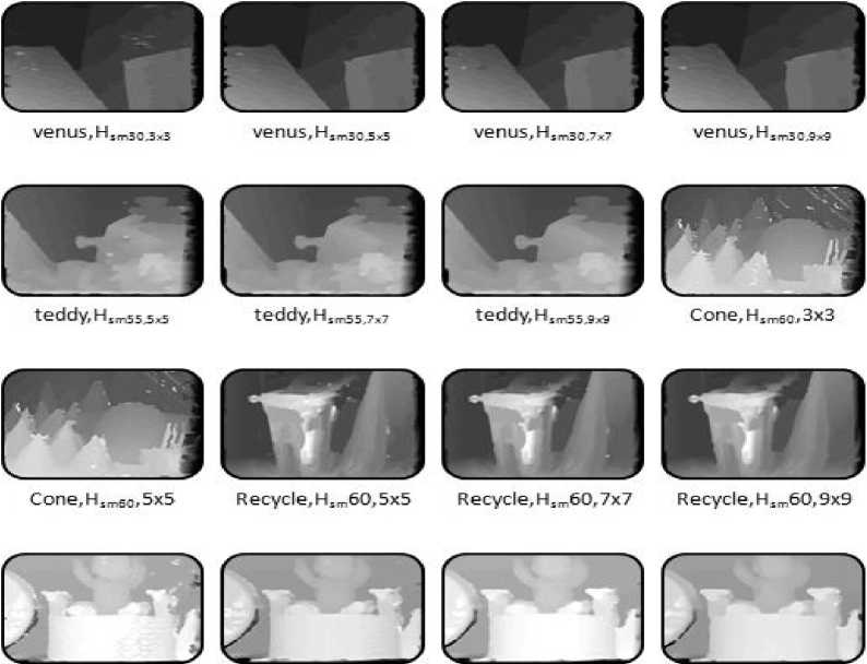
Fig.6. The results of depth and SSIM map using rgbtoxyz conversion

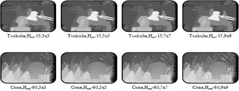
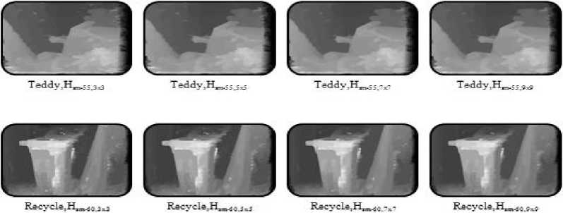
Fig.7. The result of depth and ssim map using rgbtolab conversion

Fig. 6 shows the results of venus, teddy, cone and baby depth map using rgb2xyz conversion. Fig. 7 shows the results of tsukuba, teddy, cone and recycle depth map using rgb2lab conversion. Fig. 6 and 7 shows the smooth depth map because guided filter is used to reduce sharp transitions, incorrect matching and de-noise the images. The experiments show that using the morphological permutation, the noise in the depth is removed and number of holes after hole filling operation are reduced as shown in fig. 6 and 7. Morphological operator a dilation operation enlarges a region, while erosion reduces the size. A closing operation can close up internal holes in a region and smooth the contours of image. An opening operator removes the regions of an image that can’t contain structuring element. For zero depth map assignment we count the disparity map whose disparity is not defined. Therefore our algorithm is produce, low noise, reliable, robust matching, accuracy in pixel classification and smooth depth map.

• V.    Conclusion

  MatLab has been chosen for implementing proposed stereo matching algorithms. The specification of our PC is Intel Core i3-3227U CPU with 1.90 GHz working frequency, 4 GB ram PC configuration. Our results show that the proposed algorithm displays better depth map than existing algorithm shown in fig. 4 and fig. 5. Our algorithm displays better values of PSNR. We have computed SSIM value for stereo images and have observed that our algorithm computes higher SSIM value than shown in fig. 5 and fig. 6. For most of the images the average value of SSIM that we have obtained is nearer to 0.9 which is almost very close to the ground truth images. The algorithm improve the accuracy at depth discontinuities by applying guided filtering, zero depth mapping, hole filling and morphological permutation. The experimental result on Middlebury test set identifies the performance of proposed method that is comparable with the current stereo matching algorithms. The depth maps recovered by our algorithm are close to the ground truth data. Quality metrics are used for measurement of the performance of proposed algorithms and comparing our result with other algorithms. Depth maps are effectively generated by implementing proposed stereo matching algorithms, but still there is a scope for improvement. Our algorithm can be implemented to obtain a better real time performance as compared to other reported algorithm.

Acknolodgement