An Identification of Better Engineering College with Conflicting Criteria using Adaptive TOPSIS

Author: T. Miranda Lakshmi, V. Prasanna Venkatesan, A. Martin
Journal: International Journal of Modern Education and Computer Science (IJMECS) @ijmecs
Article in issue: 5 vol.8, 2016.
Free access
Students like to find better engineering college for their higher education. It is very challenging to find the better engineering college with conflicting criteria. In this research, the criterion such as academic reputation and achievements, infrastructure, fees structure, location, quality of the faculty, research facilities and other criterion are considered to find the better engineering college. Multi Criteria Decision Making (MCDM) is the most well known branch of decision making under the presence of conflicting criteria. TOPSIS is one of the MCDM technique widely applied to solve the problems which involves many number of criteria. In this research, TOPSIS is Adaptive and applied to find better engineering college. To evaluate the proposed methodology the parameters such as time complexity, space complexity, sensitivity analysis and rank reversal are considered. In this comparative analysis, better results are obtained for Adaptive TOPSIS compared to COPRAS.
Multi Criteria Decision Making (MCDM) evaluation, TOPSIS, Adaptive TOPSIS, better engineering college, COPRAS, Rank reversal, repeated ranking
Short address: https://sciup.org/15014863
IDR: 15014863
Text of the scientific article An Identification of Better Engineering College with Conflicting Criteria using Adaptive TOPSIS
Published Online May 2016 in MECS
Decision making becomes an integral part in our daily lives and will be used for complex problems including problems with multiple conflicting criteria. Multi-criteria decision making (MCDM) is a well-known decision making process based on the progression of using methods and procedures of multiple conflicting criteria into the planning process. In other words, MCDM refers to making decision in the presence of multiple, numerous and usually that involve conflicting numbers of criteria. MCDM provides a step by step procedure for which a consensus decision can be made by a group of decision makers. This well-defined procedure can reduce the amount of arguments or conflicts involved. MCDM plays an important role in solving complex problems. The development of MCDM discipline is closely related to the advancement of computing technology. With this development, it is possible to conduct systematic analysis of complex MCDM problems. Furthermore, the extensive use of computing software has generated a huge amount of information, which makes MCDM increasingly important and useful in supporting decision making.
Multi-criteria decision making aims at selecting the "best" alternative from a set of alternatives which satisfy all the criteria. In order to select the best alternative many MCDM techniques are used and applied in various applications. In this research, most widely used MCDM technique, TOPSIS is Adaptive and compared with COPRAS method. To evaluate the proposed work, Adaptive TOPSIS and COPRAS method is likely to be applied in ranking the engineering colleges.
The rest of the paper is set out as follows. In section 2, the relative literature are reviewed, section 3 describes research approach and design, section 4 describes the proposed methodology , section 5 describes the experimental design, section 6 presents the result and discussion, and finally ended up with the conclusion, the findings of the study and the future research.
-
II. Prior Research
“Decision making is the study of identifying and choosing alternatives based on the values and Preferences of the decision maker. Making a decision implies that there are alternative choices to be considered, and in such a case it not only used to identify as many of these alternatives as possible but to choose the one that best fits with our goals, objectives, desires, values, and so on”[1]
Zeleny (1982) opens his book “Multiple Criteria Decision Making” with a statement, “It has become more and more difficult to see the world around us in a onedimensional way and to use only a single criterion when judging what we see”. Multi-criteria decision making (MCDM) aims at selecting the "best" alternative from a set of alternatives which have to satisfy multiple objectives characterized by different criteria.
MCDM also referred as:
-
1. Multi-Criteria Decision Analysis (MCDA).
-
2. Multi-Dimensions Decision Making (MDDM).
-
3. Multi-Objective Decision Making (MODM).
-
4. Multi-Attributes Decision Making (MADM).
Alternatives: Alternatives represent the different choices of action or entities available to the decision maker. Usually, the set of alternatives is assumed to be finite, ranging from several to hundreds.
Criteria: Criteria represent the different dimensions from which alternatives can be viewed
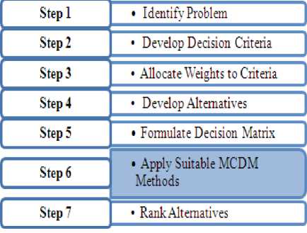
Fig.1. Multi Criteria Decision Making Process
-
A. TOPSIS
The Technique for Order Preference by Similarity to Idea Solution (TOPSIS) was first developed by Hwang and Yoon in 1981. It is relatively easy and fast, and it is most widely used method with a systematic procedure. This method is based on notation that the chosen alternative should have the shortest Euclidean distance from the ideal solution [2]. The positive-ideal solution is a solution that maximizes the benefit criteria and minimizes the cost criteria, whereas the negative ideal solution maximizes the cost criteria and minimizes the benefit criteria. Many researchers have made the comparative study of TOPSIS method with other Re345method in specific domain because of its simplicity and easiness to use. The First Step of TOPSIS Method is Normalization. Normalization has been used to deal with incongruous criteria dimension. Some of the normalization methods for TOPSIS is mention by [3]. Two methods for normalizing ratings are introduced, Gaussian normalization method and Decoupling normalization method by (Jin and Si, 2004).
Chen and Hwang, 1992 transformed Hwang and Yoon, 1981’s method into a fuzzy case. This fuzzy TOPSIS method offered a fuzzy relative closeness for each alternative, and the closeness was badly distorted and over exaggerated because of the reason of fuzzy arithmetic operations. Ref. [5] have proposed methodology consists of 3 stages: Identification of the criteria to be used in the model, FAHP computation and Ranking the alternative using VIKOR, TOPSIS, ELECTRE and PROMETHEE. The Weight of the criteria is computed using FAHP method. This paper compares the four methods to choose the best alternative among the various popes material in Sugar industry. The Result of VIKOR Method is compared with TOPSIS, ELECTRE and PROMETHEE.
Ref. [6] compares AHP and TOPSIS method using Fuzzy approach for supplier selection process. Fuzzy AHP is more appropriate than the Fuzzy TOPSIS when the purpose is to replace the supplier. Ref. [7] proposed a new approach AHP and GA method with TOPSIS to determine the quality value of cotton fiber in the textile industry. The Result of GA – TOPSIS approach was found to be the best method. [8] present a comparison of VIKOR and TOPSIS methods, which are based on distance measures. The focus of the comparison is on the properties of the aggregating function as well as on the normalization. Ref. [9] has compared six methods Weighted Sum Method (WSM), Weighted Product Method (WPM), VIKOR, PROMETHEE and TOPSIS for building design selection problem. Additionally, a method PEG – Theorem is employed. This method is a bit different from other method and it doesn’t require any preference information form the decision maker [20], [21].
Ref. [10] has taken five material selection problems. These problems are solved using common MCDM method namely, VIKOR, TOPSIS, ELECTRE. It is found that among the three, VIKOR method is best in ranking performance. Ref. [11] made a comparison on ELECTRE, TOPSIS, PROMETHEE and VIKOR method for the seismic retrofit decision problem. The comparison is made based on the ease of applicability, reliability and robustness of the choice, degree of decision maker’s influence on the results. Table 2.1 describes the Techniques combined and compared with TOPSIS [12].
-
■ Working Procedure of TOPSIS
Step 1: Construct normalized decision matrix by using the vector normalization method.
a r = for i = 1,…,m;
√∑ а j=1,…,n (1)
Where, a is the original rating of the decision matrix and r is the normalized value of the decision matrix.
Step 2: Construct the weighted normalized decision matrix by assigning different value (weight) to each criteria.
v = w ∗r for i = 1,…,m; j=1,…,n (2)
Where w the weight for j is is the criterion.
Step 3: Determine the Positive Ideal Solution (PIS) & Negative Ideal Solution (NIS).
∗ ={ v ∗ ,v ∗ ,v ∗ ,...,v ∗ } ,(3)
Where v ∗ ={ max(v ) if j⋲ ; min(v ) if j⋲
={ v ,v ,v ,...,v } ,(4)
Where v ={ min(v ) if j⋲ ; max(v ) if j⋲
Step 4: Calculate the Distance of each alternative by applying the Euclidean Distance method.
The distance from Positive Ideal Solution is:
D ∗
√∑(v ∗ - ∗ )
for i=1,…,m
Similarly, the distance from Negative Ideal Solution is:
D
= √∑(v
- )
for i=1,…,m
Step 5: Calculate the relative closeness to the ideal solution C .
D∗
C = D + D ∗
Step 6: Rank the alternatives by selecting the alternative with C closest to 1.
-
B. COPRAS
In 1996, Zavadskas and Kaklauskas created this method. It is used for evaluation of minimizing and maximizing criteria. A single criterion cannot give a full shape of the goal pursed by various clients. The COmplex PRoportional ASsessment (COPRAS) method is prioritizing the alternative on the basics of several criteria along with associated criteria weights. Ref. [13] uses a step wise ranking and evaluating procedure of the
-
■ Working Procedure for COPRAS
The COPRAS method [15] uses a stepwise ranking and evaluating procedure of the alternatives in terms of significance and utility degree. The procedure of the COPRAS method consists of the following steps:
Step 1: Selecting the set of the most important attributes, describes the alternative.
Step 2: Construct the Decision Matrix alternative in terms of significance and utility degree. The degree of utility for each alternative is shown as a percentage from 0 to 100 %. The percentage shows whether the alternative is worst or best than the other existing alternatives [14]. Ref. [13] said problems with multiple attributes are often too large for a decision maker to comprehend in their entirety.
Table 1. Comparison of Characteristic between TOPSIS and COPRAS
|
S. No |
Characteristic |
TOPSIS |
COPRAS |
|
1 |
Category |
MADM |
MADM |
|
2 |
Core process |
Positive Ideal Solution and Negative Ideal Solution |
Minimization Index and Maximization Index |
|
3 |
Attribute |
Given |
Given |
|
4 |
Normalization technique used |
Vector normalization |
Vector normalization |
|
5 |
Weight Elicitation |
Given |
Given |
|
6 |
No of alternative and attributes |
Many more |
Many more |
|
7 |
Ranking |
Ranking based on Relative Closeness Coefficient |
Ranking based on Utility Degree |
X
X X=
Х
X
X
X
Х
Х
Y лпш
Where stands for the number of alternatives, m stands for the number of the attributes.
Step 3: Determining the weight of the attributes q
Step 4: Normalization of the Decision Making Matrix x̅ by
x
̅x̅̅ = for i = 1,…,n;
∑ x for j = 1,…,m; (2)
Where j attribute in the th alternative of a solution; m is the number of attributes; n is the number of the alternatives compared. Normalized decision-making matrix
|
^^^^^^^ Х̅ |
^^^^^^^ Х̅ |
^^^^^^^ Х |
|
|
^^^^^^^ Х̅ = Х |
^^^^^^^ Х̅ |
^^^^^^^ Х̅ |
(3) |
|
^^^^^^^ Х̅ |
^^^^^^^ Х̅ |
^^^^^^^ Х |
|
Step 5: Calculation of the Weighted Normalized Decision Matrix ̂Х .
Х = x̅ . q for i = 1,…,n;
for j = 1,…,m; (4)
Weighted Normalized decision-making matrix:
|
Х̂ |
̂Х |
Х |
|
|
̂Х = Х |
Х̂ |
̂Х |
(5) |
|
̂ |
|||
|
Х̂ |
̂Х |
Х |
|
Step 6: Calculate maximization index of the alternative.
P = ∑ x̂ (6)
Step 7: Calculate minimization index of the alternative.
R = ∑ x̂
Step 8: Calculation of the relative weight of each alternative Q .
Q = P +
∑ .
Step 9: Calculation of the utility degree of each alternative.
N = ∗ 100
J Qmax
Where Q and Q are the significance of projects obtained from Eq. (8).
-
C. Findings of the Survey
MCDM has many methods which capture much attention from researchers in evaluating, accessing and ranking the alternatives in different applications. Numerous MCDM methods are developed to solve the real – world decision problems. TOPSIS method is widely used which work to satisfactorily across different application area. Since many applications are evaluated using TOPSIS method. This method is not applied in evaluating the college selection process. From the survey it also found that only limited work made a comparative study on TOPSIS method with COPRAS method.
-
■ It is possible to combine (hybrid) TOPSIS with other kinds of MCDM method. From the literature review very limited work has been found to simplify the TOPSIS.
-
■ Since there are many normalization techniques, only vector normalization is used in TOPSIS method.
-
■ From the literature it is found that TOPSIS steps have not been Adaptive.
-
■ Sensitivity analysis is the parameter which is most widely used in evaluating the efficiency of the MCDM method.
In order to make the steps easy the generalized TOPSIS steps are compressed. On simplifying this TOPSIS method it will obtain a lesser amount of time and space complexity. To find the efficiency of the proposed work, COPRAS method is compared with Adaptive TOPSIS. The evaluation parameters, Sensitivity analysis and ranking reversal are performed where it has found that Adaptive TOPSIS is more efficient than COPRAS method.
-
III. Research Approach And Design
MCDM is used to evaluate different optimal and feasible criteria to choose the best alternative. It contains many methodology among those TOPSIS is one of the well known and the most acceptable methodology. The Adaptive- TOPSIS methodology is introduced in the proposed work to improve the ranking efficiency of the algorithm in an efficient manner. There are many normalization techniques where TOPSIS contains only vector normalization. In Adaptive TOPSIS the normalization is change into linear sum based normalization. To evaluate the proposed approach it is applied in the ranking the engineering college. The decision matrix is formulated for ranking. The formulated matrix is applied in the Adaptive TOPSIS and COPRAS method. This Adaptive – TOPSIS method is compared with COPRAS method, in the direction of finding the better MCDM Method. The best MCDM Method among Adaptive TOPSIS and COPRAS is evaluated based on the performance of these methodologies Time Complexity (Big O) and Space Complexity, Sensitivity Analysis and Ranking Reversal. When comparing these algorithms, the proposed approach attains better performance.
-
IV. Proposed Methodology
TOPSIS is most widely used method among many MCDM techniques. TOPSIS was developed by Hwang and Yoon in 1981. In Generalized TOPSIS method, there is an individual step for every process. In the proposed work, the TOPSIS method is Adaptive. In general, TOPSIS method uses vector normalization to normalize the decision matrix, whereas the Adaptive TOPSIS methodology uses Gaussian normalization to normalize the raw values of the decision matrix [4]. Similarly, the stepwise procedure for generalized TOPSIS method is Adaptive in order to make the process easy.
-
A. Working Procedure for Adaptive –TOPSIS
Step 1: Construct normalized decision matrix by using the linear sum based normalization method.
Ri (j) = "Г (1)
√∑7=1 Aj
Where A j stands for the rating for criteria j
Step 2: Calculate the Distance of each alternative by applying the Euclidean Distance method. The distance from Positive Ideal Solution is:
Di — √∑ 7=1 ((wj∗ Ri(j)) -max(wj∗ Ri(j)))
for i = 1,2,…,m (2)
Similarly, the distance from Negative Ideal Solution is:
DiZ √∑ 7=1 ((w ∗ Ri(j)) -min(w ∗ Ri(j))) for i = 1,2,…,m (3)
Step 3: Calculate the relative closeness to the ideal solution Ci.
D
C 1------
Step 4: Ranking the alternatives by selecting the alternative with C i closest to 1
-
V. Experimental Design
-
A. Dataset Collection
There are wide ranges of colleges and they offer many course. But most of the student prefers to go to engineering, making a decision about the correct engineering college to choose from many options that are available. The question then arises of how to decide a college when there are thousands of engineering colleges in India. For selecting the best engineering college student may look for different criteria’s. Based on those criteria they will select the best college and course. The data is collected from post graduate student about the 17 engineering in Cuddalore and Puducherry. 14 criteria are taken for evaluating the college. The average data are calculated to formulate the decision matrix. Table 2 shows original matrix.
Table 2. Original Decision Matrix
|
C 1 |
C 2 |
C 3 |
C 4 |
C 5 |
C 6 |
C 7 |
C 8 |
C 9 |
C 1 0 |
C 1 1 |
C 1 2 |
C 1 3 |
C 1 4 |
|
|
A 1 |
4 |
3 |
3 |
2 |
3 |
3 |
3 |
3 |
3 |
3 |
3 |
2 |
4 |
3 |
|
A 2 |
4 |
4 |
3 |
3 |
3 |
3 |
3 |
4 |
3 |
3 |
3 |
3 |
3 |
3 |
|
A 3 |
3 |
2 |
3 |
3 |
3 |
3 |
3 |
2 |
3 |
2 |
3 |
3 |
2 |
3 |
|
A 4 |
3 |
3 |
3 |
3 |
3 |
3 |
2 |
3 |
3 |
3 |
3 |
3 |
3 |
3 |
|
A 5 |
3 |
2 |
3 |
3 |
3 |
3 |
2 |
3 |
3 |
2 |
3 |
3 |
3 |
3 |
|
A 6 |
4 |
4 |
3 |
3 |
4 |
3 |
4 |
3 |
3 |
4 |
3 |
4 |
2 |
3 |
|
A 7 |
4 |
5 |
4 |
4 |
4 |
4 |
3 |
4 |
4 |
4 |
4 |
3 |
4 |
4 |
|
A 8 |
4 |
5 |
5 |
4 |
5 |
4 |
4 |
4 |
4 |
4 |
4 |
5 |
4 |
4 |
|
A 9 |
4 |
4 |
4 |
3 |
4 |
3 |
3 |
4 |
4 |
3 |
3 |
4 |
4 |
3 |
|
A 1 0 |
3 |
3 |
3 |
3 |
3 |
3 |
3 |
2 |
2 |
3 |
3 |
3 |
3 |
3 |
|
A 1 1 |
3 |
3 |
3 |
2 |
3 |
3 |
3 |
3 |
2 |
3 |
2 |
3 |
3 |
3 |
|
A 1 2 |
2 |
3 |
3 |
3 |
2 |
3 |
3 |
3 |
3 |
3 |
3 |
3 |
3 |
3 |
|
A 1 3 |
3 |
3 |
3 |
3 |
3 |
3 |
3 |
3 |
3 |
3 |
3 |
3 |
3 |
3 |
|
A 1 4 |
4 |
3 |
3 |
3 |
3 |
3 |
3 |
3 |
2 |
3 |
3 |
3 |
4 |
3 |
|
A 1 5 |
3 |
3 |
3 |
3 |
3 |
3 |
3 |
2 |
3 |
3 |
3 |
3 |
1 |
3 |
|
A 1 6 |
3 |
3 |
3 |
3 |
2 |
3 |
2 |
3 |
1 |
3 |
3 |
3 |
2 |
3 |
|
A 1 7 |
4 |
4 |
4 |
3 |
3 |
4 |
3 |
4 |
4 |
4 |
4 |
4 |
4 |
3 |
The weights for the criteria play an important role where it normalizes the decision matrix. Table 3 shows the weights for the criteria.
Table 3. Weights for Criteria
|
Criteria |
Weight ( Wj ) |
|
Academic Reputation/ Ranking of the College |
0.7735 |
|
Academic Achievements (Gold Medal, Top Ranks etc.) |
0.8031 |
|
Infra structure |
0.7337 |
|
Fees Structure |
0.6163 |
|
Location of the college |
0.6449 |
|
Quality of the faculty |
0.7541 |
|
Research facilities |
0.6408 |
|
Placement facilities |
0.8245 |
|
Placement track record |
0.7898 |
|
Extra-curricular activities |
0.6153 |
|
Co-curricular activities |
0.6051 |
|
Transport facilities |
0.7306 |
|
Hostel facilities |
0.6561 |
|
Personal safety of the student |
0.7061 |
The positive ideal solution and the negative ideal solution obtained from the weighted normalized decision matrix are as follows:
POSITIVE IDEAL SOLUTION = {0.0690, 0.0877, 0.0893, 0.0392, 0.0926, 0.0741, 0.0800, 0.0755, 0.0800, 0.0755, 0.0755, 0.0909, 0.0769, 0.0755}
NEGATIVE IDEAL SOLUTION = {0.0345, 0.0351, 0.0536, 0.0784, 0.0370, 0.0556, 0.0400, 0.0377, 0.0200, 0.0377, 0.0377, 0.0364, 0.0192, 0.0566}
Table 4. PIS and NIS, Relative Closeness Coefficient and ranking for Adaptive TOPSIS
|
Alternatives |
Distance ( D/ ) |
Distance ( ПГ ) |
RCC (Ci ) |
Rank |
|
A1 |
0.0702 |
0.0688 |
0.4950 |
7 |
|
A2 |
0.0593 |
0.0707 |
0.5439 |
6 |
|
A3 |
0.0845 |
0.0458 |
0.3514 |
16 |
|
A4 |
0.0709 |
0.0546 |
0.4352 |
10 |
|
A5 |
0.0801 |
0.0515 |
0.3911 |
13 |
|
A6 |
0.0546 |
0.0752 |
0.5793 |
5 |
|
A7 |
0.0421 |
0.0983 |
0.7003 |
2 |
|
A8 |
0.0242 |
0.1131 |
0. 8239 |
1 |
|
A9 |
0.0405 |
0.0904 |
0.6908 |
4 |
|
A10 |
0.0775 |
0.0464 |
0.3747 |
14 |
|
A11 |
0.0743 |
0.0520 |
0.4117 |
11 |
|
A12 |
0.0760 |
0.0532 |
0.4115 |
12 |
|
A13 |
0.0673 |
0.0561 |
0.4545 |
9 |
|
A14 |
0.0703 |
0.0611 |
0.4648 |
8 |
|
A15 |
0.0808 |
0.0476 |
0.3708 |
15 |
|
A16 |
0.0906 |
0.0369 |
0.2896 |
17 |
|
A17 |
0.0401 |
0.0935 |
0.7000 |
3 |
In the same way, the original decision matrix and weights from the Table 2 and Table 3 is applied in COPRAS method. The COPRAS method also ranked the first college as A8: Pondicherry University, Pondicherry. This college is ranked first, because the utility degree value is 100% when compared with other college. Table 5 shows the Utility degree and ranking order of the college.
Table 5. Utility degree and ranking of an alternative using COPRAS
|
Alternative |
Utility degree (N ) |
Rank |
|
A1 |
70.11 % |
8 |
|
A2 |
75.46% |
6 |
|
A3 |
63.24 % |
16 |
|
A4 |
68.42 % |
10 |
|
A5 |
65.18% |
13 |
|
A6 |
78.17 % |
5 |
|
A7 |
91.87 % |
2 |
|
A8 |
100 % |
1 |
|
A9 |
83.89 % |
4 |
|
A10 |
66.08 % |
12 |
|
A11 |
65.08 % |
14 |
|
A12 |
66.85 % |
11 |
|
A13 |
70.04 % |
9 |
|
A14 |
71.32 % |
7 |
|
A15 |
64.89% |
15 |
|
A16 |
61.33 % |
17 |
|
A17 |
87.05 % |
3 |
On comparing the result from Adaptive TOPSIS and COPRAS method both Adaptive TOPSIS and COPRAS method ranks Pondicherry University as a best college. In this research, the MCDM methods are implemented in MATLAB version7.9.0.529 (R2009b). The collected data has been processed in MATLAB.
-
VI. Results And Discussion
By comparing the Multi Criteria Decision making methodology, COPRAS with the proposed methodology Adaptive TOPSIS the following results are obtained. Two methods Adaptive TOPSIS and COPRAS are implemented with the same input to obtain the best and the worst alternative. The ranking of Adaptive TOPSIS and COPRAS method are compared by the parameters. Each parameter is applied in both the method in order to find the better method. The efficiency of algorithm is determined by the following two metrics.
-
a) Computation time of the algorithm (Time Complexity)
-
b) Space required by the algorithm (Space Complexity)
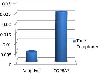
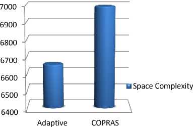
Table 6. Time and Space Complexity in S-TOPSIS and COPRAS
|
Methods |
Time complexity (seconds) |
Space complexity (bytes) |
|
Adaptive TOPSIS |
0.005072 |
6656 |
|
COPRAS |
0.025635 |
6992 |
Table 6 describes the Time and Space Complexity of Adaptive TOPSIS and COPRAS. From the results it is observed that the Adaptive TOPSIS has taken limited computation time and space complexity.
TOPSIS
MCDM Methods
Fig.2. Time Complexity of Adaptive TOPSIS and COPRAS
TOPSIS
MCDM Methods
-
Fig.3. Space Complexity of Adaptive TOPSIS and COPRAS
Figure 2 shows diagrammatical view of Adaptive TOPSIS which has less time complexity. Where, figure 3 shows diagrammatical view of Adaptive TOPSIS which has less space complexity than COPRAS method.
-
A. Sensitivity An alysis
Sensitivity analysis measures the impact on the outcome by changing one or more key input values. Sensitivity analysis is used to investigate how sensitive the ranking of alternatives when changes in weights and belief degrees for certain attributes [18]. Hence, performing a Sensitivity Analysis on the results of a decision problem may provide valuable information to the decision maker about the robustness of the solution. The sensitivity analysis is conducted in different way by using weight. Generally, the total sum of the weight is always equal to one. That is the range of weight is from 0.1 to 0.9. The Sensitivity analysis is conducted in Adaptive TOPSIS and COPRAS method to check robustness of the solution in these methods. Sensitivity analysis can be performed by changing weights in different method. The weights are change in two different methods and the efficiency is checked.
-
■ Assign all attributes a weight value of 1, called basic weight.
-
■ Sensitivity analysis on exchanging each criterions weight with another criterions weight [19].
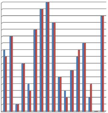
The Adaptive TOPSIS and COPRAS method are performed by changing all the weights of the criteria to 1. The result of sensitivity analysis is shown in below table when all the weights have changed to 1. From the Table 7 it has shown that the rank for the alternatives is changing in Adaptive TOPSIS when conducting Sensitivity analysis. The alternatives are A5 – A7 – A10 – A17.
In the same way, Sensitivity Analysis is conducted in COPRAS method. The rank of the following alternative is getting changed in this method. The alternatives are A1 – A11 – A13 – A15. On seeing the result of sensitivity analysis, the ranking of both methods are changing equally when all the criteria’s weights are changed to 1. Figures 4 and Figure 5 have clearly shown that the rank of both Adaptive TOPSIS and COPRAS are changing equally when weights are change to 1.
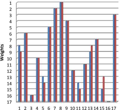
Then the Sensitivity analysis on exchange each criterions weight with another criterion weight is conducted. Table 8 shows the result of sensitivity analysis on exchanging weights. From the Table 8 the rank for the following alternatives is changed in Adaptive TOPSIS when conducting Sensitivity analysis. The alternatives are A5 – A7 – A9 – A10 – A17. In the same way, Sensitivity Analysis is conducted in COPRAS method.
The rank of the following alternative is getting changed in this method. The alternatives are A1 – A5 – A11 – A13 – A16. On seeing the result of sensitivity analysis, the ranking of both methods are changing equally when all the criteria’s weights are exchanged. But the best alternative in both the method doesn’t get changed. The Sensitivity Analysis is conducted in two different ways where both the method the ranking result from both Adaptive TOPSIS and COPRAS method are changing equally.
Table.7. Sensitivity analysis in Adaptive TOPSIS and COPRAS when all the weights are 1
|
Alternatives |
Adaptive TOPSIS |
COPRAS |
||||||
|
Before |
After |
Before |
After |
|||||
|
RCC |
RANK |
RCC |
RANK |
RCC |
RANK |
RCC |
RANK |
|
|
A1 |
0.4950 |
7 |
0.5046 |
7 |
70.11% |
8 |
70.06% |
9 |
|
A2 |
0.5439 |
6 |
0.5284 |
6 |
75.46% |
6 |
74.96% |
6 |
|
A3 |
0.3510 |
16 |
0.3539 |
16 |
63.24% |
16 |
63.53% |
16 |
|
A4 |
0.4352 |
10 |
0.4323 |
10 |
68.42% |
10 |
68.39% |
10 |
|
A5 |
0.3911 |
13 |
0.3897 |
14 |
65.18% |
13 |
65.14% |
13 |
|
A6 |
0.5793 |
5 |
0.5788 |
5 |
78.17% |
5 |
78.31% |
5 |
|
A7 |
0.7003 |
2 |
0.6834 |
3 |
91.87% |
2 |
91.73% |
2 |
|
A8 |
0.8239 |
1 |
0.8006 |
1 |
100% |
1 |
100% |
1 |
|
A9 |
0.6908 |
4 |
0.6765 |
4 |
83.89% |
4 |
82.33% |
4 |
|
A10 |
0.3747 |
14 |
0.3932 |
13 |
66.08% |
12 |
66.71% |
12 |
|
A11 |
0.4117 |
11 |
0.4242 |
11 |
65.08% |
14 |
64.96% |
15 |
|
A12 |
0.4115 |
12 |
0.4111 |
12 |
66.85% |
11 |
66.98% |
11 |
|
A13 |
0.4545 |
9 |
0.4563 |
9 |
70.04% |
9 |
70.18% |
8 |
|
A14 |
0.4648 |
8 |
0.4765 |
8 |
71.32% |
7 |
71.64% |
7 |
|
A15 |
0.3708 |
15 |
0.3685 |
15 |
64.89% |
15 |
65.06% |
14 |
|
A16 |
0.2896 |
17 |
0.2931 |
17 |
61.33% |
17 |
61.45% |
17 |
|
A17 |
0.7000 |
3 |
0.6871 |
2 |
87.05% |
3 |
86.60% |
3 |
Sensitivity Analysis (Adaptive TOPSIS)
Sensitivity Analysis (COPRAS)
,м '5
1 2 3 4 5 6 7 8 9 1011121314151617
Alternatives
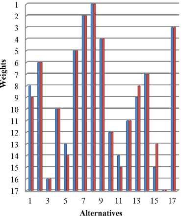
Fig.5. Sensitivity Analysis on changing weights to 1 for COPRAS
Fig.4. Sensitivity Analysis on changing weights to 1 for Adaptive TOPSIS
In Adaptive TOPSIS, 4 ranks are getting changed when Sensitivity analysis is conducted by changing all the weights to 1. And 5 ranks are getting changed when Sensitivity Analysis is conducted on exchanging weights. In the same way, for COPRAS method, 4 ranks are getting changed when Sensitivity analysis is conducted by changing all the weights to 1. And 5 ranks are getting changed when Sensitivity Analysis is conducted on exchanging weights. But the best alternative doesn’t get changed in both the method. Both the result shows that the proposed method Adaptive TOPSIS is efficient and compared method COPRAS also efficient when this parameter is applied.
Table 8. Sensitivity analysis in Adaptive TOPSIS and COPRAS when the weights are exchanged
|
Alternatives |
Adaptive TOPSIS |
COPRAS |
||||||
|
Before |
After |
Before |
After |
|||||
|
RCC |
RANK |
RCC |
RANK |
RCC |
RANK |
RCC |
RANK |
|
|
A1 |
0.4950 |
7 |
0.5046 |
7 |
70.11% |
8 |
70.06% |
9 |
|
A2 |
0.5439 |
6 |
0.5284 |
6 |
75.46% |
6 |
74.96% |
6 |
|
A3 |
0.3510 |
16 |
0.3539 |
16 |
63.24% |
16 |
63.53% |
16 |
|
A4 |
0.4352 |
10 |
0.4323 |
10 |
68.42% |
10 |
68.39% |
10 |
|
A5 |
0.3911 |
13 |
0.3897 |
14 |
65.18% |
13 |
65.14% |
13 |
|
A6 |
0.5793 |
5 |
0.5788 |
5 |
78.17% |
5 |
78.31% |
5 |
|
A7 |
0.7003 |
2 |
0.6834 |
3 |
91.87% |
2 |
91.73% |
2 |
|
A8 |
0.8239 |
1 |
0.8006 |
1 |
100% |
1 |
100% |
1 |
|
A9 |
0.6908 |
4 |
0.6765 |
4 |
83.89% |
4 |
82.33% |
4 |
|
A10 |
0.3747 |
14 |
0.3932 |
13 |
66.08% |
12 |
66.71% |
12 |
|
A11 |
0.4117 |
11 |
0.4242 |
11 |
65.08% |
14 |
64.96% |
15 |
|
A12 |
0.4115 |
12 |
0.4111 |
12 |
66.85% |
11 |
66.98% |
11 |
|
A13 |
0.4545 |
9 |
0.4563 |
9 |
70.04% |
9 |
70.18% |
8 |
|
A14 |
0.4648 |
8 |
0.4765 |
8 |
71.32% |
7 |
71.64% |
7 |
|
A15 |
0.3708 |
15 |
0.3685 |
15 |
64.89% |
15 |
65.06% |
14 |
|
A16 |
0.2896 |
17 |
0.2931 |
17 |
61.33% |
17 |
61.45% |
17 |
|
A17 |
0.7000 |
3 |
0.6871 |
2 |
87.05% |
3 |
86.60% |
3 |
Sensitivity Analysis on Exchanging weights for Adaptive TOPSIS
Sensitivity Analysis on Exchanging weights for COPRAS
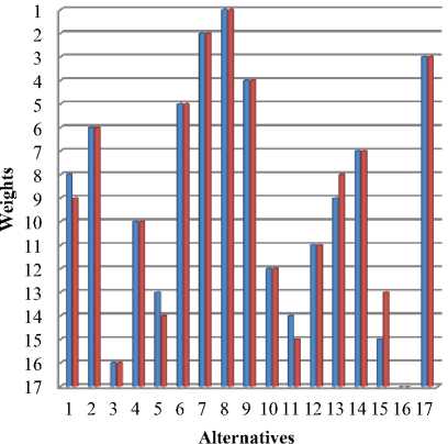
Fig.6. Sensitivity Analysis on Exchanging weights for Adaptive TOPSIS
Alternatives
Fig.7. Sensitivity Analysis on Exchanging weights for COPRAS
-
B. Rank Reversal
Rank reversal means that the ranking between two alternatives might be reversed after some variation occurs to the decision problem, like adding a new alternative, dropping an old alternative or replacing a non-optimal alternative by a worse one etc. Usually such a rank reversal is undesirable for decision-making problems. If a method does allow it to happen, the validity of the method could be questioned. Rank reversal of adding and removing the alternatives are taken for evaluation [20]. And they are applied in Adaptive TOPSIS and COPRAS method to check the efficiency.
The new alternative 18 is introduced in the original data. The Relative Closeness Coefficient and ranks obtain before and after rank reversal is shown in the below Table 9. On conducting the Rank Reversal for Adaptive TOPSIS and COPRAS the best rank in both the method doesn’t get changed on adding a new alternative. The Table 9 has shown that the rank reversal issues in both the method are limited and no changes in the best alternative even the new alternative is added.
Figure 8 and Figure 9 have clearly shown that the best alternative doesn’t get change. The rank remains same for the following alternative A7 - A8 - A12 - A17 in Adaptive TOPSIS. Then for COPRAS method the rank remains same for A7 – A8.
Table 9. Rank Reversal in Adaptive TOPSIS and COPRAS for adding a new Alternative
|
Alternativ es |
Adaptive TOPSIS |
COPRAS |
||||||
|
Before |
After |
Before |
After |
|||||
|
RCC |
RANK |
RCC |
RANK |
RCC |
RANK |
RCC |
RANK |
|
|
A1 |
0.4950 |
7 |
0.5046 |
7 |
70.11% |
8 |
70.06% |
9 |
|
A2 |
0.5439 |
6 |
0.5284 |
6 |
75.46% |
6 |
74.96% |
6 |
|
A3 |
0.3510 |
16 |
0.3539 |
16 |
63.24% |
16 |
63.53% |
16 |
|
A4 |
0.4352 |
10 |
0.4323 |
10 |
68.42% |
10 |
68.39% |
10 |
|
A5 |
0.3911 |
13 |
0.3897 |
14 |
65.18% |
13 |
65.14% |
13 |
|
A6 |
0.5793 |
5 |
0.5788 |
5 |
78.17% |
5 |
78.31% |
5 |
|
A7 |
0.7003 |
2 |
0.6834 |
3 |
91.87% |
2 |
91.73% |
2 |
|
A8 |
0.8239 |
1 |
0.8006 |
1 |
100% |
1 |
100% |
1 |
|
A9 |
0.6908 |
4 |
0.6765 |
4 |
83.89% |
4 |
82.33% |
4 |
|
A10 |
0.3747 |
14 |
0.3932 |
13 |
66.08% |
12 |
66.71% |
12 |
|
A11 |
0.4117 |
11 |
0.4242 |
11 |
65.08% |
14 |
64.96% |
15 |
|
A12 |
0.4115 |
12 |
0.4111 |
12 |
66.85% |
11 |
66.98% |
11 |
|
A13 |
0.4545 |
9 |
0.4563 |
9 |
70.04% |
9 |
70.18% |
8 |
|
A14 |
0.4648 |
8 |
0.4765 |
8 |
71.32% |
7 |
71.64% |
7 |
|
A15 |
0.3708 |
15 |
0.3685 |
15 |
64.89% |
15 |
65.06% |
14 |
|
A16 |
0.2896 |
17 |
0.2931 |
17 |
61.33% |
17 |
61.45% |
17 |
|
A17 |
0.7000 |
3 |
0.6871 |
2 |
87.05% |
3 |
86.60% |
3 |
|
A18 (new) |
||||||||
Table 10. Rank Reversal in Adaptive TOPSIS and COPRAS for removing the worst Alternative
|
Alternatives |
Adaptive TOPSIS |
COPRAS |
||||||
|
Before |
After |
Before |
After |
|||||
|
RCC |
RANK |
RCC |
RANK |
RCC |
RANK |
RCC |
RANK |
|
|
A1 |
0.4950 |
7 |
0.4724 |
7 |
70.11% |
8 |
70.06% |
9 |
|
A2 |
0.5439 |
6 |
0.5284 |
6 |
75.46% |
6 |
74.96% |
6 |
|
A3 |
0.3510 |
16 |
0.3539 |
16 |
63.24% |
16 |
63.53% |
16 |
|
A4 |
0.4352 |
10 |
0.4323 |
10 |
68.42% |
10 |
68.39% |
10 |
|
A5 |
0.3911 |
13 |
0.3897 |
14 |
65.18% |
13 |
65.14% |
13 |
|
A6 |
0.5793 |
5 |
0.5788 |
5 |
78.17% |
5 |
78.31% |
5 |
|
A7 |
0.7003 |
2 |
0.6834 |
3 |
91.87% |
2 |
91.73% |
2 |
|
A8 |
0.8239 |
1 |
0.8006 |
1 |
100% |
1 |
100% |
1 |
|
A9 |
0.6908 |
4 |
0.6765 |
4 |
83.89% |
4 |
82.33% |
4 |
|
A10 |
0.3747 |
14 |
0.3932 |
13 |
66.08% |
12 |
66.71% |
12 |
|
A11 |
0.4117 |
11 |
0.4242 |
11 |
65.08% |
14 |
64.96% |
15 |
|
A12 |
0.4115 |
12 |
0.4111 |
12 |
66.85% |
11 |
66.98% |
11 |
|
A13 |
0.4545 |
9 |
0.4563 |
9 |
70.04% |
9 |
70.18% |
8 |
|
A14 |
0.4648 |
8 |
0.4765 |
8 |
71.32% |
7 |
71.64% |
7 |
|
A15 |
0.3708 |
15 |
0.3685 |
15 |
64.89% |
15 |
65.06% |
14 |
|
A16 |
0.2896 |
17 |
0.2931 |
17 |
61.33% |
17 |
61.45% |
17 |
|
A17 |
0.70000 |
3 |
0.6871 |
2 |
87.05% |
3 |
86.60% |
3 |
Rank Reversal for adding alternative in Adaptive TOPSIS
Rank Reversal on removing an alternative in Adaptive TOPSIS
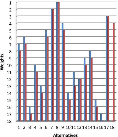
Fig.8. Rank Reversal for adding alternative in Adaptive TOPSIS
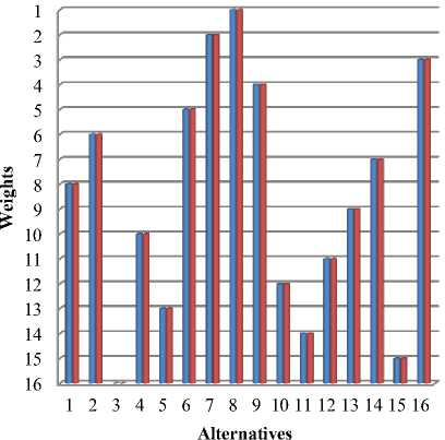
Fig.10. Rank Reversal on removing an alternative in Adaptive TOPSIS
Rank Reversal on removing an alternative in COPRAS
Rank Reversal for adding alternative in COPRAS
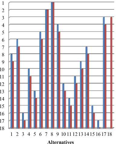
Fig.9. Rank Reversal for adding alternative in COPRAS
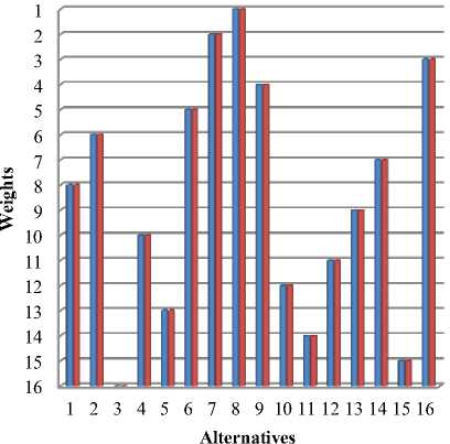
Fig.11. Rank Reversal on removing an alternative in COPRAS
On conducting the Rank Reversal for Adaptive TOPSIS and COPRAS the best rank in both the method doesn’t get changed on removing the worst alternative. Table 10 has shows the result of Adaptive TOPSIS and COPRAS method before and after removing the alternative. The rank remains same for the following alternative A1 - A2 - A3 - A6 - A7 – A8 – A9 – A12 – A13 – A14 – A15 – A17 in Adaptive TOPSIS. And for COPRAS method all ranks remains same. The above Figure 10 and Figure 11 show the rank reversal on removing the alternative.
-
C. Evaluation of Adaptive TOPSIS
The Adaptive TOPSIS is evaluated using the following parameters: Time and Space Complexity, Sensitivity analysis and Rank Reversal. The result obtain from Time and Space complexity from Table 6 shows that both complexity are less in Adaptive TOPSIS on comparing with COPRAS method. The time complexity in Adaptive TOPSIS is 0.005072 seconds and the space complexity is 6656 bytes. Then the sensitivity analysis is conducted in two different methods. The weights for all the criteria are changed to 1 and the weights for all the criteria’s are exchanged with each other. Both the methods of sensitivity analysis are applied in Adaptive TOPSIS and COPRAS method. The result from sensitivity analysis is shown in Table 7 and Table 8. The Figure 4 and Figure 5 show the pictorial representation of the result on conducting sensitivity analysis by changing all the weights to 1. And Figure 6 and Figure 7 show the result of sensitivity analysis on exchanging weights. The result on conducting sensitivity analysis shows that the proposed method Adaptive TOPSIS and COPRAS method performs equally. Both the result shows that the proposed method Adaptive TOPSIS is efficient.
Finally, Rank Reversal is conducted in Adaptive TOPSIS and COPRAS method. The rank reversal is conducted by adding and removing the alternative. The Rank reversal results are shown in Table 9 and Table 10. According to the result of Adaptive TOPSIS method, A8 is the best among the 17 alternatives. Since the ranking is slightly different from the rank obtain before ranking reversal. It is no wonder that different methods may produce slightly different rankings. The best alternative A8 is not getting changed. Then the worst alternative A 1 6 is dropped out of the original alternative set which is shown in Table 10. The best alternative A8 remains same. The rank in Adaptive TOPSIS and COPRAS method are doesn’t get reversed when an alternative is added or removed.
-
VII. Conclusion
Multi Criteria Decision Making is widely used for decision making problem where there are several factors in obtaining the best solution and different methods are used for solving complex problem. The problem is to rank the engineering college in Cuddalore and Puducherry. Many algorithms are available in MCDM where TOPSIS is one of the most preferred on when compared to other methods. The proposed work introduces a new MCDM approach which Simplifies TOPSIS method. The performance of the proposed method, Adaptive TOPSIS is compared with COPRAS method. The efficiency of algorithms is measured in terms of Time and space complexity, Sensitivity Analysis and Rank Reversal. The Proposed method, Adaptive TOPSIS attains a better result with time and space complexity, Sensitivity Analysis and Rank Reversal. As a result of the comparative analysis on Adaptive TOPSIS with COPRAS method, the proposed method attains better result. In future, Adaptive TOPSIS method can be compared with other Multi Criteria Decision Making methods. The efficiency of the algorithms can be evaluated with other parameters.
References An Identification of Better Engineering College with Conflicting Criteria using Adaptive TOPSIS
- Fülöp. J, "Introduction to Decision Making Methods," pp. 1–15, 2001
- Athawale. V. M and Chakraborty. S, "A comparative study on the ranking performance of some multi-criteria decision-making methods for industrial robot selection," Int. J. Ind. Eng. Comput., vol. 2, no. 4, pp. 831–850, Oct. 2011.
- Shih H.S, "Incremental analysis for MCDM with an application to group TOPSIS," Eur. J. Oper. Res., vol. 186, no. 2, pp. 720–734, Apr. 2008.
- Lansing. E and Si. L, "A Study of Methods for Normalizing User Ratings in Collaborative Filtering." The 27th annual international ACM SIGIR Conference, Sheffield, pp. 568-569, 2004.
- Anojkumar. L, Ilangkumaran. M, and Sasirekha. V, "Comparative analysis of MCDM methods for pipe material selection in sugar industry," Expert Syst. Appl., vol. 41, no. 6, pp. 2964–2980, May 2014.
- Lima Junior. F. R, Osiro. L, and Carpinetti L. C. R, "A comparison between Fuzzy AHP and Fuzzy TOPSIS methods to supplier selection," Appl. Soft Comput., vol. 21, pp. 194–209, Aug. 2014.
- Banwet D. K and Majumdar. A, "Comparative analysis of AHP-TOPSIS and GA-TOPSIS methods for selection of raw materials in textile industries," pp. 2071–2080, 2014.
- Opricovic. S and Tzeng. G.-H, "Compromise solution by MCDM methods: A comparative analysis of VIKOR and TOPSIS," Eur. J. Oper. Res., vol. 156, no. 2, pp. 445–455, Jul. 2004.
- Mela. K, Tiainen. T, and Heinisuo. M, "Comparative study of multiple criteria decision making methods for building design," Adv. Eng. Informatics, vol. 26, no. 4, pp. 716–726, Oct. 2012.
- Chakraborty. S and Chatterjee. P, "Selection of materials using multi-criteria decision-making methods with minimum data," Decis. Sci. Lett., vol. 2, pp. 135–148, Jul. 2013.
- Caterino. N, Iervolino. I, Manfredi. G, and Cosenza. E, "A Comparative Analysis of Decision Making Methods for the Seismic Retrofit of RC Buildings," 2008.
- Behzadian. M, Otaghsara. S. K, Yazdani. M, and Ignatius. J, "Expert Systems with Applications A state-of the-art survey of TOPSIS applications," Expert Syst. Appl., vol. 39, no. 17, pp. 13051–13069, 2012.
- Zavadskas. L, Kaklauskas, Sakalauskas and G. W. Weber, "Contractor selection multi-attribute model applying copras method with grey interval numbers," 2008.
- Misra. S. K and A. Ray, "Comparative Study on Different Multi-Criteria Decision Making Tools in Software project selection scenario," vol. 3, no. 4, pp. 172–178, 2012.
- Zavadskas E. K., A. Kaklauskas, Z. Turskis, and J. Tamosaitiene, "Selection of the effective dwelling house walls by applying attributes values determined at intervals," J. Civ. Eng. Manag., vol.s 14, no. 2, pp. 85–93, Jan. 2008.
- Podvezko. V, "The Comparative Analysis of MCDA Methods," vol. 22, no. 2, pp. 134–146, 2011.
- Dey, D. N. Ghosh, and A. C. Mondal, "A MCDM Approach for Evaluating Bowlers Performance in IPL," vol. 2, no. 11, pp. 563–573, 2011.
- Alinezhad and Amini, "Sensitivity Analysis of TOPSIS Technique: The Results of Change in the Weight of One Attribute on the Final Ranking of Alternatives," vol. 7, pp. 23–28, 2011.
- Chen, C. Liao, and L. Wu, "A Selection Model to Logistic Centers Based on TOPSIS and MCGP Methods: The Case of Airline Industry," vol. 2014.
- Ying-Ming Wang and Ying Luo, "On Rank reversal in decision analysis", Mathematical and Computer Modelling, vol. 49, pp 1221-1229, March 2009.
- Sreenivasa Rao Basavala, Narendra Kumar, and Alok Agarrwal, "Finding Vulnerabilities in Rich Internet Applications (Flex/AS3) Using Static Techniques," International Journal of Modern Education and Computer Science (IJMECS), vol. 4, no. 1, pp. 33-39, February 2012.
- Miranda Lakshmi, T., Martin, A., Mumtaj Begum, R., V. Prasanna Venkatesan. "An Analysis on Performance of Decision Tree Algorithms using Student's Qualitative Data." International Journal of Modern Education & Computer Science 5, no. 5 (2013).
