An Improved Particle Swarm Optimization for Protein Folding Prediction

Published Online February 2011 in MECS

• I.    I NTRODUCTION

  Protein can play normal physiological function [1] when amino acid sequence forms a particular three dimensional structure. Therefore, understanding the structure of protein is important to study the function of it. Using computer simulation to predict protein structure, based on the theory that native conformation of proteins is the lowest free energy conformation, was proposed by Anfinsen in 1973 [2]. We predict protein conformation by simulating protein folding process [3]. This method is current research focus because of simplicity and less constraints. Researchers proposed simplified mathematical models of protein based on the fact that hydrophobic residues are wrapped inside by hydrophilic residues and hydrophilic residues expose to the surface which contacts with water [4]. Among them, AB off-lattice model is more accurate proposed by Stillinger [5, 6] since this model not only takes into account the hydrophobic and hydrophilic, but also makes chemical bonds between amino acids changeable and determines the protein conformation through the perspective of the adjacent chemical bonds. Therefore, AB off-lattice model has no position constraint and reflects protein structure.

Protein fold prediction based on AB off-lattice model is a typical NP problem, and many optimization algorithms have been applied to this problem, such as ant colony optimization [7], tabu search algorithm [8], genetic-annealing algorithm [9], neural network algorithm [10] and so on. Particle Swarm optimizer (PSO), which was proposed in 1995 by Eberhart and Kennedy [11] based on foraging behaviors of birds, has advantages in solving continuous optimization problems because of its simplicity, convenience, fast convergence and fewer parameters so that been often chosen to solve protein fold prediction problems. However, PSO has poor convergence precision and easily to trap into local optimum. So this paper introduces levy flight into PSO and combines PSO and Levy Flight which has better local search ability to improve convergence rate and algorithm’s efficiency.

In section II, we present an overview of AB off-lattice model. Then we give an introduction of Particle Swarm Optimizer (PSO), random process – Levy Flight and the proposed algorithm (LPSO) in section III. In section IV, we show the results obtained by the new algorithm from the experiments and compare its performance to the basic Particle Swarm Optimizer. Section V is our conclusion.

• II.    P ROTEIN M ODEL

At present, the pervasive method to predict the structure of proteins is simulating their formation process through computer, which is merely in the initial stage. Therefore, the model of protein folding prediction is hoped that it can not only reflect the main features of real protein structure, but also make the computer simulation practicable, which lead a contradiction between model’s accuracy and simplicity. Researchers have put forward some simplified models [12,13], such as full-atom model, HP lattice model and AB off-lattice model, among which we choose the third one for the continuous bond angles in this model are arbitrary so it can simulate protein structure more truly.

AB off-lattice model, proposed by Stillinger in 1993 ， divided amino acids into hydrophobic amino acids (A) and hydrophilic amino acids (B) based on strength of the affinity between amino acids and water.

• A.    2D AB Off-Lattice Model

First of all, we give a simple introduction to AB off-lattice model in 2D space, which is similar to HP lattice model and divides amino acids into two categories, i.e. hydrophobic amino acid (A) and hydrophilic amino acid (B).

Two amino acids connect through rigid bond, which eventually lead to the formation of non-direction linear polymer. We can determine the structure of n amino acids polypeptide chain through n-2 bond angles, i.e. θ 2 , ⋯ , θ n-1 , where -π< θ i <π. Additional, when θ i equals to zero, it means that two continuous bonds are on the same line.

Amino acids are clockwise turning when 9 i <0 and obviously, 9 i >0 represents counterclockwise rotation, as Fig.1 shows.

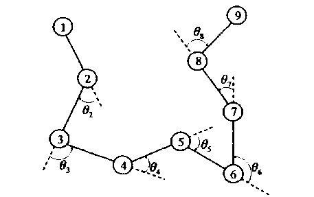
Figure 1. 2D AB Off-Lattice Model

• B.    3D AB Off-Lattice Model

According to 2D model, we can get the model is 3D space, i.e. 3D AB off-lattice model. It simplified complex amino acids sequence to sequence containing A and B and predicts protein conformation according to bond angle and bond energy between amino acids. Bond angles ( 9 ) in 2D AB off-lattice model are transformed to horizontal bond angles ( a ) and dimensional angles ( p ) in 3D model. A protein sequence containing n amino acids contains n-2 horizontal bond angles a ₂, ..., a i , ..., a _n- 1 (2 <  i <  n-1) and n-3 three dimensional angles p ₃, ..., P j , ..., p _n-1 (3 < j < n-1), where a i =0 shows three adjacent amino acids are on the same line and if amino acids are clockwise turning, a _i is larger than 0, or a _i is smaller than 0.

Protein energy function contains two parts, one is the bending potential energy of protein backbone (E 1 ), and the other is gravitational potential energy between nonadjacent amino acids (E 2 ). E 1 depends on adjacent chemical bonds’ angles while E 2 depends on distances between non-adjacent amino acids and the affinity between amino acids and water. The potential function E of a protein sequence with n amino acids can be defined as the following equations.

n -1                  n -2 n

E = 2E1(«,) + XS E2(jSi,Si)

i = 2                  i = 1 j = i + 2

E1 (ai) = 4(1 - cos ai)

E2( j Si, S,) = 4 •   - C (Si S j]

^{+ 1}

C ( S i , S j ) = <+ 0.5

- 0.5

S i = 1, S j = ¹

S i =- 1, S _} =- 1

Si * Sj

Here r_i j represents the Euler Distance between the ith amino acids and the jth amino acids. We define the distance between two adjacent amino acids as 1, so r_i j depends on a and p . ^ i =1 if amino acids belong to A while ^ i =-1 if amino acids belong to B.

In this paper, we set the initial position of amino acids sequence at the initial point P1(0, 0, 0) of three dimensional coordinate system and the second amino acids at X axis so the position is P2(1, 0, 0). Then we put the third amino acids at XOY plane and others in threedimensional space. We use 9i to denote the projection included angle between the extend line of corresponding amino acids and adjacent amino acids in XOY plane (the same in 2D model), as Fig.2 shows. As mentioned previously, pi is the angle between corresponding amino acids and XOY plane, as Fig.3 shows. So we can use 9i and pi to calculate cos ai and the ith amino acids’ position which is (xi, yi, zi). Among them, i-1

xi = xi-1 + cosC^ 9k)cos Д-1, k=2

i - 1

• < yt= y t_x + sin(2 9k )cos A-1, k=2

zi = zi-1 + sin Pi-1.

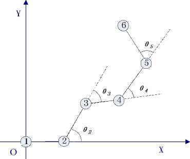
Figure 2. Amino acids’ projection in XOY plane

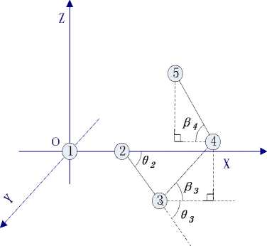
Figure 3. Amino acids’ coordinate graph

the optimization problem). Each particle uses its own experience and the experience of neighbor particles to choose how to move in the search space. Therefore, at each step, particles update themselves by tracking personal best position (pbest) and global best position (gbest or lbest). For the gbest model, each particle shares information with all the particles in the search space. However, for the lbest model, each particle exchanges information with its neighborhood particles. In this paper, we use the gbest model of Particle Swarm Optimizer to solve protein folding prediction. Each particle updates its velocity and position according to (2) and (3). Let Xi = ( Хи, X . ₂,--’ X D ) T represent the ith particle’s position and V = ( v. 1 , v. 2 ,..., V D ) represent the ith particle’s velocity.

• ^V (,, + 1 ) = wv (,, )⁺ c l r 1 ( Pbe^St ( i, ) — x ( it ) )

Therefore, r_i j can be calculated by the positions of P_i and P j , which is VOj-xd+ty-yJ+Z -З ².

uuur

Let vector V represents P i-1 pointing to P i which is

(x_i-x_i-1, y_i-y_i-1, z_i-z_i-1). Then the angle α _i can be calculated as follow:

uuur uur uuur uur cos a = (V г V)/ V i ■ V .

I I — 1 I I — 1 I

Since all the points’ positions can be denoted by 9 and P according to (1), r ij and cos a i can be calculated.

Then the problem of predicting protein conformation through AB off-lattice model is changed to the process that getting the minimum of the potential function E by changing 9 i and p i , i.e., can be expressed as follows:

minij_„ ) E (б2_,™,9„ ™,Pn_„

A,-™ Pj,™, Pn _1)

• III.    L EVY F LIGHT P ARTICLE S WARM O PTIMIZATION

• A.    Particle Swarm Optimizer

  Particle Swarm Optimizer (PSO), based on the behavior simulations of birds and fish proposed by Eberhart and Kennedy in 1995 [11], shows that a single individual usually doesn’t have intelligence, but the whole swarm always has the ability in handling complex problems. PSO was originally used to deal with continuous optimization problems, but it has been extended to combinatorial optimization problems. Particle Swarm Optimizer was originally designed as a numerical optimization technique based on swarm intelligence, and it has shown its robustness and efficacy for solving function-value optimization problems in real-number spaces. Due to its simplicity and efficiency, many researchers have focused on this field.

At the beginning, PSO initializes a group of particles randomly (each particle represents a candidate solution to

⁺ c 2 r 2 ( gbest ( g., ) — ^X ( i,t ) )

• X (i,,+1) = X (i,,) + V (i,,+1) (3)

Let w denote the inertia weight while v ( _{i, t+1} ) denote the ith particle’s velocity at (t+1)th iteration. c ₁ and c ₂ are learning factors. c ₁ is self-learning factor while c ₂ is society learning factor. c ₁ and c ₂ adjust to the maximum step size of flight to personal best position and global best position. If c ₁ and c ₂ are too small, particles may fly away the target area. By contraries, if c ₁ and c ₂ are too great, particles suddenly fly to the target area or fly over the target area. r ₁ and r ₂ are random numbers between 0 and 1. x ( _{i , t+1} ) is the ith particle’s position at (t+1)th iteration. pbest ( _{i, t} ) is the ith particle’s personal best position (pbest). gbest ( _{g, t} ) is global best position (gbest). To prevent particles from exceeding the search space, each particle’s velocity is limited between - V_max and V_max . Generally, V_max shouldn’t exceed particle’s width range. If V_max is too great, particles will fly away from the best solution. Or this may reduce particle’s global search ability and cause particles trapping in local optima. Particles’ positions at each dimension are also limited between - X_max and X_max .

According to (1), the velocity of the particle at each iteration can be calculated using three terms: the velocity of the particle at the previous iteration, the distance of particle from its best previous position and the distance from the best position of the entire population. Therefore, the particle flies to a new position according to (2). The maximum number of iterations is usually used for the PSO algorithm’s termination condition.

• B.    LevyFlight

Levy flights are a special class of random walks whose step lengths are not constant but rather are chosen from a probability distribution with a power-law tail. This method of simulation stems heavily from the mathematics related to chaos theory. Chaotic transport is studied experimentally in two-dimensional flow in a rapidly rotating annular tank. And levy flights are useful in stochastic measurement and simulations for random or pseudo-random natural phenomena [14], signals analysis as well as many applications in astronomy, biology and physics. Realizations of levy flights are physical phenomena, but now much of interest is concentrated on whether we can find levy flights in biological systems.

Random processes can be seen everywhere in nature. The normal and anomalous random processes are ubiquitous in many branches of physics, chemistry, biology, economics and other science. The most famous jump-type stochastic process is called as levy flight, in the process of which the traveling particle undergoes a random sequence of some short jumps, intermittently broken by a single or merely a few long steps.

A levy flight, named after the French mathematician Paul Pierre Levy [15], is type of random walk in which the increments are distributed according to a heavy-tailed probability distribution. Specially, the distribution used is a power law of the form y = x ^-a where 1 <  a <  3 and therefore has an infinite variance [16]. In recent years, more and more researchers pay their close attention to levy-stable distribution, because levy fight can be represented by levy stable distribution [17]. Levy stable distribution has a rich class of probability distribution that allows skewness and fat tails and has many interesting mathematical properties.

• C.    LPSO

Particle Swarm Optimizer is an iterative optimization tool. Due to it is easy to understand and implement, PSO develops rapidly and has been widely used in many fields. It has advantages in solving continuous optimization problems because of simplicity, convenience, fast convergence and fewer parameters. Therefore, many researchers choose PSO to solve protein fold prediction problems. However, it has poor convergence precision and is easy to trap into local optimum.

Levy flight essentially provides a random walk while the random step length is drawn from Levy distribution which has an infinite variance with an infinite mean. Here the steps essentially from a random walk process with a power-law step-length distribution with a heavy tail [18]. The local search will be sped up, because some of the new solutions are generated by Levy walk around the best solution obtained so far. However, a substantial fraction of the new solutions should be generated by far field randomization and whose locations should be far enough from the current best solution, this will make sure the system will not be trapped in a local optimum.

In this paper, we introduce Levy Flight into basic PSO and propose levy flight Particle Swarm Optimizer (LPSO). In the process of levy flight the traveling particle undergoes a random sequence of some short jumps, intermittently broken by a single or merely a few long steps [19]. This is the biggest advantage of levy flight and this can help particles escape from local optimum. The algorithm proposed in this paper has better performance than basic PSO. The process is given in algorithm 1.

Step 1: Initialize all the particles’ velocities and initial positions (population size is n);

Step 2: Choose 20 particles with worse fitness;

Step 3: Update the chose particles’ postions and velocities by random process - Levy Flight;

Step 4: Evaluatte all the particles;

Step 5: Update paticles’ personal be st positions (pbest);

Step 6: Update swarm’s global best positions (gbest);

Step 7: Update particles’ velocities and positions by Equation (1) and Equation (2);

Step 8: Determine the termination condition (usually set a certain evaluation generations). If not achieve the end condition, return Step4; Or end the algorithm.

Algorithm 1. Process of LPSO

In our algorithm, we select 20 particles from the entire population and generate new positions and velocities for these 20 particles by levy flight. If the new position of a particle is better than the original position, this particle will be reinitialized with the new position and velocity and its personal best memory will be deleted. However, if the new position is not better than the original position, the particle will be not initialized. In this paper, we run the levy flight every c steps. This is because each particle needs a number of generations to locate the global optimum. If we use levy flight to reinitialize particles’ positions and velocities, these particles cannot determine which position is more probably to locate the global optimum. The greatest advantage of reinitializing particles using levy fight is to void particles trapping into local optimum. If a particle trapped into local optimum, the proposed algorithm could help this particle fly away the local optimum by updating its position and velocity with levy flight. Pseudo code of our algorithm is given in algorithm 2.

F or iteration < maxGeneration do

If iteration % c == 0

Choose 20 particles with worse ftness;

Generate new positions and velocities by random process - Levy Flight;

For eachparticle in the 20 chose particles

If new position betrer than original position

Update this particle's position;

Update this particle's velocity;

End If

End For

End If

Algorithm 2. Pseudo code of LPSO

C. Results

For all the particles

Calculate each particle's fitness;

If ph e st < current fitness

Update this particle's personal best position (pbest);

End If

End For

Update population's global best position;

Update each particle's velocity by Equation (1);

Update each particle's position by Equation (2);

End For

Continued Algorithm 2. Pseudo code of LPSO

• IV.    E XPERIMENT AND A NALYSIS

• A.    Experiment

• 1)    Fibonacci sequence, which is defined in (4), is widely used in protein fold prediction.

S 0 = A, S 1 = B, ⋯ , S i+1 = S i-1 * S i                     (4)

Where ‘*’ is connection symbol. So S2 = AB, S3 = BAB and so on. Let A denote hydrophobic amino while B denote hydrophilic amino.

• 2)    We downloaded four real protein sequences from the PDB database ( http://www.rcsb.org/pdb/home/home . do) as follow:

2KGU:GYCAEKGIRCDDIHCCTGLKCKCNASGNC VCRKK

1CRN:TTCCPSIVARSNFNVCRLPGTPEAICATYT GCIIIPGATCPGDYAN

2KAP:KEACDWLRATGFPQYAQLYEDFLFPIDIS LVKREHDFLDRDAIEALCRRLNTLNKCAVMK

1PCH:AKFSAIITDKVGLHARPASVLAKEASKFSS NITIIANEKQGNLKSIMNVMAMAIKTGTEITIQADG NDADQAIQAIKQTMIDTALIQG

Where D, E, F, H, K, N, Q, R, S, T, W and Y are hydrophilic amino acids while I, V, L, P, C, M, A and G are hydrophobic ones.

• B.    Parameters

  In this paper, for all the algorithms, number of particles are 100. Maximum iteration is 2000. c1 and c2 are both equal 2.05. Inertia weight w is 0.9. We ran all the experiments for 50 times and calculated the lowest energies.

The proposed algorithm in this paper used the version of constraint factor. If any particle with a position x_i exceeds the boundary of solution space, its position will be reset to a value that is twice of the boundary subtracting x_i .

TABLE 1. Lowest Energies of Fibonacci sequence

Length	Sequence	PSO	LPSO
5	ABBAB	-0.2182	-1.0627
8	BABABBAB	-1.2856	-2.0038
13	ABBABBABABBAB	-2.8218	-4.6159
21	BABABBABABBAB BABABBAB	-4.1515	-6.6465
34	ABBABBABABBAB BABABBABABBAB BABABBAB	-4.2235	-7.3375
55	BABABBABABBAB BABABBABABBAB BABABBABBABAB BABABBABBABAB BAB	-8.0209	-13.0487

Table 1 shows the lowest energy of PSO and LPSO in solving Fibonacci sequence with different length. Form it we can see that the lowest energy of the length of 5, 8, 13, 21, 34 and 55 got by PSO are -0.2182, -1.2856, -2.8218, -4.1515, -4.2235 and -8.0209 respectively. However, the lowest energy of the same length got by our algorithm are -1.0627, -2.0038, -4.6159, -6.6465, -7.3375 and -13.0487. So we can conclude that LPSO can always get lower energy without reference to the length of Fibonacci sequence.

Fig.4-Fig.6 show the simulated diagram of Fibonacci sequence with length 13, 21 and 34 predicted by LPSO, in which black spot represents hydrophobic amino acid residues (A) while white spot represents hydrophilic amino acid residues (B). These figures can be used for predicting the structures of proteins sequence and satisfy the properties of protein. That shows the feasibility of the proposed algorithm in this paper.

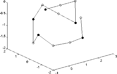
Figure 4. Fibonacci sequence with length 13

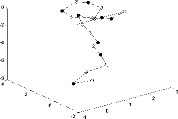
Figure 5. Fibonacci sequence with length 21

• Fi gure 6. Fibonacci sequence with length 34

TABLE 2 shows lowest energy of PSO and LPSO in solving four real protein sequences in database PDB, which are 2KGU, 1CRN, 2KAP and 1PCH. From TABLE2, we can see that the lowest energies are -8.3635, -20.1826, -8.0448 and -18.4408 respectively by PSO. However, the proposed algorithm in this paper can get -20.9633, -28.7591, -15.9988 and -46.4964 in solving these sequences. From it we can see that LPSO has lower energy than basic PSO and we can conclude than LPSO has better performance in solving real protein sequences.

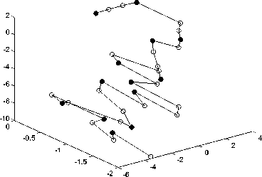
TABLE 2. Lowest energies of real protein sequence

Name	PSO	LPSO
2KGU	-8.3635	-20.9633
1CRN	-20.1826	-28.7591
2KAP	-8.0448	-15.9988
1PCH	-18.4408	-46.4964

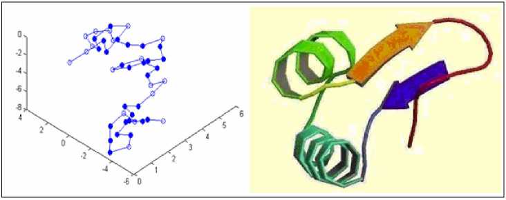
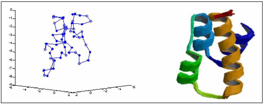
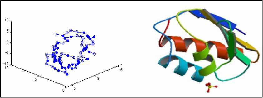
Fig.7-Fig.10 shows the structures of real protein sequences predicted by LPSO and the real structures in the PDB database. In each Figure, (a) shows the results of LPSO while (b) shows the real structure. From these four figures, we can see that the structures predicted by LPSO are similar to the native conformation of proteins. Therefore, LPSO is a feasible solution for protein folding prediction.

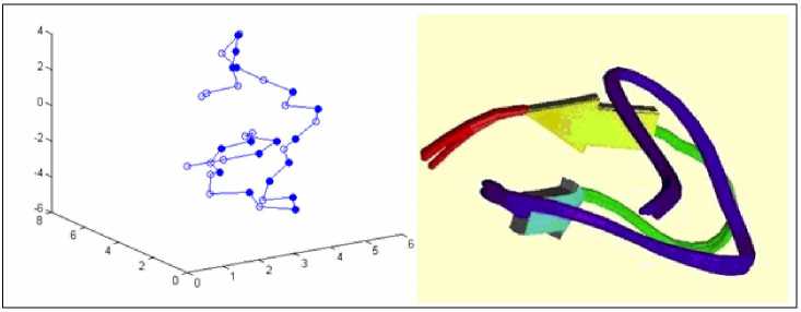
(a) 2KGU predicted by LPSO

(b) 2KGU in PDB

Figure 7. Comparison of 2KGU

(a) 1CRN predicted by LPSO

(b) 1CRN in PDB

Figure 8. Comparison of 1CRN

(a) 2KAP predicted by LPSO

(b) 2KAP in PDB

Figure 9. Comparison of 2KAP

(a) 1PCH predicted by LPSO                                 (b) 1PCH in PDB

Figure 10. Comparison of 1PCH

• V.    C ONCLUSION

In this paper we use an improved PSO with levy flight to solve the problem of Protein Folding Prediction. Particle Swarm Optimizer converges fast and has strong global search capability. While the traveling particle undergoes a random sequence of some short jumps in the process of levy flight, intermittently broken by a single or merely a few long steps. It is the biggest advantage of levy flight and can help particles escape from local optimum. So we combine PSO and levy flight and propose a new algorithm called LPSO, which we used to solve Protein Folding Prediction problem based on threedimensional AB off-lattice model. Experiments show that LPSO has better performance than basic PSO so it is a feasible solution for this problem.

However, the proposed algorithm in this paper needs more computation cost and more function evaluations in solving simple problems. In the future, we will focus on reducing the computation cost to shorten the running time, such as using parallel processing and running the algorithm on GPU.

A CKNOWLEDGMENT

The authors wish to thank Ren Lan for his previous work in this problem. We also thank anybody who helped us in our paper.