Анализ ультразвуковых изображений узлов щитовидной железы с помощью метода извлечения характеристик изображения

DOI:

Thyroid nodules are a relatively common clinical condition, almost always benign, though sometimes an early indication of more serious pathologies, including thyroid cancer. Recent studies indicate that thyroid nodules are diagnosed in about 69% of adults undergoing thyroid ultrasound. Therefore, there is a critical need for accurate and efficient diagnostic tools.

With the increased incidence of thyroid nodules around the world, the case for advanced diagnostic methods becomes even more compelling [1].

Deep learning has now emerged as quite a powerful force in biomedical imaging, changing the ways of analyzing and interpreting medical images. Among many others, CNN’s have shown remarkable success in classifying and segmenting medical images with unprecedented accuracy and efficiency. Challenges, such as vast amounts of labeled data required for it to be effective, often make deep learning models associated with over-fitting that reduces their generalization to new datasets [2].

The current research deals with thyroid nodule classification and diagnosis using CNN’s and deep machine-learning techniques. In this paper, we apply transfer learning and data augmentation to overcome the challenges of small datasets, while ensuring high accuracy and robustness in our models. Our study is not only aimed at increasing diagnostic accuracy regarding thyroid nodule detection, but also providing a complete framework that could be applied to other areas of medical imaging.

Thyrotoxicosis, Graves' hyperthyroidism, and other thyroid diseases require efficient treatment. Since 2011, novel ideas have been presented to assess the anetiology of thyrotoxicosis, manage hyperthyroidism with antithyroid medications, manage prenatal highs in thyroid hormone individuals, and train candidates for surgical treatment of the thyroid, with extended portions for simpler reasons [3, 4].

It also goes on to consider the broader implications of deep learning in health care, notably its capacity for systematizing and optimally standardizing all diagnostic processes across all fields of medicine. We, therefore, hope that this work shall help add to the increasing researches using artificial intelligence to better patients' lives and shape the future of medical diagnostics [5]. Modifying CNN’s in genuine photographs improves characteristics for a variety of types of medical imaging. Such traits serve to create multi-class classification algorithms, and their past likelihoods are combined to forecast previously unknown images. This approach uses generic picture features from natural photos to improve the relevancy of the extraction of features [6, 7]. The illustration depicts the butterfly-shaped thyroid system below the middle inside the larynx towards the windpipe, featuring the thyroid nodule as well as parathyroid tissue visible from the outside, shown in the Figure 1.

In this paper, we will marry state-of-the-art deep learning with conventional approaches and open up a completely new method of thyroid nodules classification, hence enabling possibilities for more accurate and reliable diagnoses. This research underlines AI's role in modern medicine and hints at the potential these technologies hold for a transformed future of healthcare.

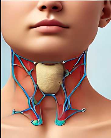
Figure 1. The Image of Thyroid Nodule.

RELATED WORK

Thyroid nodules over the past two decades, there have been a significant increase in thyroid nodule detection, leading to the accidental discovery of many nodules. Since most thyroid nodules are benign or have an indolent behavior, separating them from malignant ones with fine needle aspirations and surgical resections would save the patients a great deal of time and hassle. Radiologists can use sonography to investigate atypical thyroid nodules. Radiologists have found that hypoechogenicity, microcalcifications, hardness, and a shape that is taller than wide are all sonographic signs of cancerous thyroid nodules [8-11].

The thyroid nodules are the most common lesions in the thyroid gland and currently occur at the highest incidence in the past thirty years [12, 13]. To a certain extent, the high density and artifacts in thyroid CT images restrict traditional image processing in machine learning [14].

Nevertheless, X-ray CT is becoming increasingly essential as a diagnostic tool for a whole series of diseases related to the thyroid organ. Recent experimental investigations have revealed that the presence of noise and complexity problems within these scans does not allow traditional image-processing techniques to work well enough on such images [15, 16].

Current research has increasingly concentrated on addressing these issues. On the other hand, recent methods that leverage the recent advancements in deep learning, particularly

CNN’s, have demonstrated promisingly high performance in various medical imaging applications. Recently, there has been a significant improvement in nodule detection in chest radiographs and chest CT [17].

However, researchers have not thoroughly studied the method numerous research studies have been presented, as the density and artifacts resulting from thyroid CT images pose challenges in their assessment. E-density and artifacts resulting from them. Conventional image processing has been in practice for quite some time in identifying thyroid nodules [18, 19].

Some of the methods applied include edge detection, thresholding, and morphological processes. For instance, some of the techniques used in the identification of thyroid nodules in ultrasound images include texture analysis and morphological procedures [20, 21].

Such methods have problems with low contrast and noise, which renders results unreliable [22].

One application used U-Net to segment thyroid nodules. In this respect, the group suggested a segmentation technique dependent on annotation marks, whereby manual points guide the result of the major and minor endpoint axes of a nodule. We manually compute these axes at four locations and draw four white dots at these locations in the image. This guides the deep neural network in training and inferring a deep learning-based segmentation strategy for thyroid cancer that distinguishes thyroid nodules [23].

Another paper proposed a multi-task cascade deep learning model that performs automated thyroid nodule detection using multi-modal ultrasound data and integrates radiologists' expertise. This is basically transferring knowledge networks to get more accurate results for nodule segmentation [24]. The process then quantifies the ultrasonic features of the nodule, utilizing this information to generate stronger images and discriminators [25, 26].

The introduction of machine learning brought about significant improvements. Techniques such as support vector machines and k-nearest neighbors have been involved in thyroid nodule classification using hand-crafted features [27, 28]. The researchers used Support Vector Machine (SVM) to classify thyroid nodules and realized a fairly good level of accuracy. However, because manually created features were used, their applicability to models in a wide range of situations was limited [29]. Employing basic characteristics decreases speed and adds to the network's complexity and intricacy. Whereby a novel shade detection technique has been suggested, focusing primarily on key characteristics and examining the related data across neighboring feature levels [30].

As a result, accurate segmentation of thyroid nodules is one of the most important factors in accurate classification. It found its application in many medical image segmentation fields; variants of the U-Net model could capture intricate features accurately. An improved U-Net framework was proposed for the segmentation of thyroid nodules in ultrasound images [9, 31].

The anatomy found in the cerebral cortex is difficult to visualize utilizing standard imaging techniques. Imaging methods such as noise reduction as well as gray-level combination network retrieval assist discriminate between regular versus sick organs with flawless precision. During categorization, the Discrete Wavelet Transform (DWT) is used, while positional identification is done using conditional artificial neural network (ANN) algorithms [32, 33].

Results showed that this architecture performed better than traditional segmentation techniques. However, the above studies did not use CNN’s with sophisticated image-processing techniques to detect thyroid nodules. The present study precisely detects thyroid nodules by combining CNN with region-based image processing techniques.

MATERIAL AND METHODS

Data Collection

The Thyroid Digital Image Database, an open-access repository of 480 genuine cases of thyroid nodule conditions represented through grayscale images, represents the dataset for this research. In this instance, there were 280 cases of malignant conditions diagnosed with TIRADS scoring 4a, 4b, 4c, and 5, plus 200 cases of benign conditions diagnosed with TIRADS scoring 2 and 3. We applied image augmentation to enhance the neural network model's robustness by diversifying the images, resulting in a total of 2000 images. We then divided the images into three sets: 1000 for training, 400 for validation, and 200 for testing [34, 35].

Dataset

We divided the dataset into three parts: training, validation, and testing. The dataset sample shown in Figure 2.

• •      Training Dataset: We used the Training Dataset to train the model. To reduce

errors, the model iteratively learned from provided data by modifying its parameters.

• •      Validation Dataset: We used the validation set to fine-tune hyperparameters like

learning rate and network architecture during the training process. This avoided over-fitting; hence, the model generalized well to test data.

• •      Testing Dataset: We used the Test Dataset to objectively assess the final model's

performance at the end of training. We isolated it from training and validation datasets to assess a model's ability to generalize to new, unseen data.

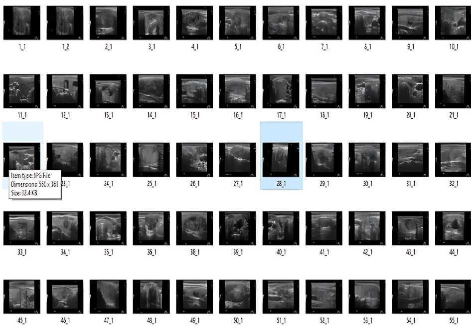
Figure 2. Dataset of Thyroid Nodule.

The process architecture of dataset is showing Figure 3.

Training Data

Validation Data

Figure 3. Dataset Process Architecture

Pre-Processing

Most importantly, we applied preprocessing to these images. The following work was completed:

The preprocessing pseudocode was as follows:

Prepare the image (X, A)

Image = X

Современные инновации, системы и технологии // Modern Innovations, Systems and Technologies 2024; 4(3)

Required size is A

Natural jpeg image input

Pre-processed png image as the output

• 1.    X for every Image

• 2.    Do

• 3.    Change the format of X to .png

• 4.    Add a 1x1 pixel black border

• 5.    Fuzz by X to 10%

• 6.    Trim X

• 7.    Re page X

• 8.    Gravity Center X

• 9.    Resize A

• 10.    X on a black background

Close loop

Return X.

• •     Image Resizing: We resized all images to 128x128 pixels and converted them into PNG

format from their original format using the GraphicsMagick toolkit.

• •     Data Cleaning: involves finding missing values and handling them properly, removing

any duplicate data.

• •      Category Conversion: The neural network model required a numerical representation of

the categorical features.

Convolutional Neural Network (CNN)

In this paper, CNN has been designed for the classification of thyroid images. It contained a few convolutional layers using filters of size 3x3, after which pooling layers were added to reduce the spatial dimensions of the feature maps. In the Figure 4, shown the use of CNN. The final layers were then connected fully and ended in a softmax output layer that classified the images into benign or malignant categories [36].

• •      Convolutional Layers: These layers convolved the input images to detect low-level

features such as edges and textures.

• •     Pooling Layers: Max-pooling was applied to down-sample the feature maps, only

retaining the most prominent features.

• •      Fully Connected Layers: These layers combined the high-level features that were

extracted by the convolutional and pooling layers before finally making the classification.

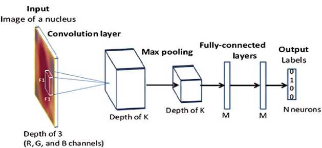
Figure 4. The CNN Using Process.

Network Architecture of VGG Net

Our training dataset consisted of input RGB images with dimensions of 128x128 pixels. We applied center cropping to the input images to obtain the necessary pixel sizes for our experiments. The images passed through a succession of convolutional layers, each using small 3x3 filter sizes. We kept the convolution stride at 1 pixel and added 1 pixel of padding to retain the spatial dimensions. In max-pooling, we used windows of 2x2 pixels with a stride of 2, and similarly, 3x3 windows with a stride of 2 [37, 38].

Next, we stack our architecture with convolutional layers and three fully connected layers, allowing us to construct diverse topologies at different depths. BoThe first two fully connected layers, each with 2048 channels, and the third fully connected layer, which classifies our five classes with 5 channels, remain structurally homogeneous throughout the network, culminating in a final layer of sigmoid or softmax for output classification. ide from that, the hidden layers have ReLU nonlinearity for activation [39, 40].

In this work, we developed and experimented with four different models of VGGNet to achieve the best performance on our dataset. The shallowest one among all the VGGNet models developed is Model A, consisting of fewer numbers of convolutional layers. We will present this model in this paper to demonstrate the network's potential for image classification [31]. VGGNet Model B increased the network's depth by introducing more convolutional layers, which further extracted features. Clearly, a deeper architecture has improved accuracy, but at the cost of more computation [41, 42].

We push it one step further with VGGNet Model C, which is much deeper—not just in the number of convolutional layers, but in terms of the number of filters within each layer. We designed this model to capture subtle changes in the images, incorporating improvements such as different activation functions and dropout rates to prevent overfitting. Model C showed major improvements in accuracy and robustness. Finally, VGGNet Model D had all the excellent features taken from the previous models, plus advanced fine-tuning methods involving batch normalization and learning rate adjustments. While this model was more complicated and computationally expensive, it ended up working best on both accuracy and generalization, making it the optimal architecture for our own classification task. This would allow us to further refine our approach so that we could be more specific about which VGGNet model works well on our dataset.

Model: "sequential"                                                                        |				Model: “sequential_l”
Layer (type)	Output Shape		Param #	layer (type)	—	Output Shape	Param #
conv2d (Conv2D)	(None, 128,     ,	M)		conv2d_4 (      ) conv2d 5 (Cori'   )	—	(None,   ■ , 128, 1 (None, ,     , ।	) )
conv2d_l (loruj.)	(None, ,    ,	-)	36,928	max pooling2d 2 (             )		(None, • ,    , 04	)
max_pooling2d (MaxPool )	(None, , i,	)	0	conv2d 6 (Con \ )		(None, 64,   , •	S)
conv2d_2 ( w2D)	(None, , ,	}	/3,856	conv2d_7 (COOVZD)		(None, ,    ,	)
conv2d_3 ( iv2D)	(None, i, 64,			max pooling2d з (             )		(None,    ,    ,    . (None,   ,   ,	5) 5)
max pooling2d 1 ( ;хРх_1	(None, , ,	!S)		conv2d_9 (Conv2D)	—	(None, ,   ,	)
flatten (Flatten)	(None, 31072)		0	max pooling2d 4 (	-K2D)	(None, ,   ,
dense (Dense)	(None, 2048)		268,437,504	Flatten! (      ,i)		(None, 6'    :)	0
dense_l (Dense)	(None, 2048)		4,196,152	dense_3 (D ) dense_4 (Dense) dense 5 (Dense)		(None, 048)	134,219,2/6
dense_2 (Dense)	(None, )		10,245		—	(None, ^mh) (None, )
Total params:              (1.02 GB) Trainable params:              (1.02 GB) Non-trainable oarams: ■ (0.00 Bl				Total params:              (532.42 MB) Trainable params:              (532.42 MB) Non-trainable params: (0.00 B)
Model: "sequential_2"                                                                      1				Model: "sequential_3"
Layer (type)	output shape		Param #	Layer (type)		Output Shape	Param #
conv2d 10 (       )	(None, ,     ,	64)	1,792	conv2d 20 (       )		(None, 1 ,     ,
conv2d_ll ( ji .zj)	(None, ,     ,	64)	15,928	conv2d 21 ( i )	ing2D)	(None, 1 ,     , (None, ,    , (None,        ,	)
max_pooling2d_5 (            )	(None, , ,	3		max pooling2d 9 ( conv2d 22 (       )			) )
conv2d_12 ( i 2D)	(None, ,    ,	)		conv2d 23 (' inW J	—	(None, 64, -i.	B)
conv2d_13 ( jnv2p)	(None, 4, 64, 1	)	147,584	max_pooling2d 10 (             )		(None, ,   ,	0__
max_pooling2d_6 ( ixPooling2D)	(None,        ,	)	0	conv2d 24 (CorivzD)		(None, ,   ,	)
conv2d_14 ( 7ПУ2О)	(None, , ,		295,168	CO11V2d_25 (С0ПУ2И)		(None, , ,	)
conv2d_15 (       )	(None, , ,	)	590,080	conv2d 26 (       )		(None, ,   ,	)
conv2d_16 (       )	(None, , ,	)	590,080	max_pooling2d_ll (             )		(None, ,   ,	s)
max_pooling2d_7 (MaxPooli--2D)	(None, , 16,	)	0	CODV2O 2/ (       J C0nv2d_28 (      ) conv2d 29 (       )	—	(None,    ,    ,   i (None,    ,    ,   1 (None,     ,     ,  ■ 1	)
conv2d 17 ( )nv2D)	(None, ,    ,	)	1,180,160		—		■)                      2 359 > 808 )
conv2d_18 ( w2D)	(None, , ,	)	7,359,808	max_pooling2d_i2 (             )		(None, , ,     )	0
conv2d_19 ( i ‘)	(None, , io,	)	2,359,808	flattens (       )		(None,     8)	0
maxjooling2d_8 (       .    )	(None, , 8, I	)	0	dense_9 (Dens*)		(None, WB)	67,110,912
flatten_2 (       )	(None, 2/68)		0	batch normalization (BatchNarmalization)		(None, 2048)	8.192
dense 6 ( > )	(None, 2048)		67,110,912	dropout_2 ( : -ou )	—	(None, 2048)
dropout (        )	(None, 2048)		0	dense IB (Dens )		(None, 048)	4,196,352
dense ? (Dense)	(None, )		4,195,352	batch normalization! (BatehNormalization)		(None, 2048)	8,192
dropout l ( сш ii)	(None, «И)		0	dropout 3 ( inonr)	—	(None, 2048)	0
dense_8 (Dens )	(None, ')		10,245	dense 11 (      )		(None, )	10,245
Total params:             (301.18 MB) Trainable params:             (301.18 MB) Non-trainable params: (0.00 B)				Total params: Trainable params: Non-trainable params:	(301.24 MB) (301.21 MB) (32.00 KB)

Figure 5. VGGNET Model.

Figure 5 depicts an example of a convolutional neural network model inspired by the widely used VGGNet architecture in image classification tasks. It is built with TensorFlow and Keras on top of an input layer supporting images in RGB (128×128 pixels). The core model has a number of convolutional layers that scan the input images using filters of size 3×3. ReLU activation functions follow these convolutional layers, adding some non-linearity to the model and enabling it to learn complex patterns [43].

We add a max-pooling layer after each set of convolutional layers to reduce the spatial dimensions of the feature maps. This has the effect of downsampling the data while keeping only higher-order features of importance. The network progressively extracts features at higher levels from images by pooling after convolutional layers [44]. The network flattens data to a one-dimensional vector after feature extraction and then passes it through fully connected or dense, layers. In the first dense layer, there are 2048 neurons, using the ReLU activation function to connect the extracted features into a more abstract representation. There is a final dense layer with as many neurons as there are classes in the classification task, along with a softmax activation function that gives out probabilities for each class in this case [45, 46].

The Adam optimizer will train it, using categorical cross-entropy as the loss function, making it suitable for multi-class classification problems. Also, a TensorBoard callback will show the training process to the user, who will be able to track such metrics as accuracy and loss in real-time. This model architecture, with its combination of convolutional and dense layers, efficiently classifies images to learning and combining features progressively from the input data.

MODEL EVALUATION METRICS

A lot of different metrics were used to make sure that the suggested CNN-based system for finding and classifying thyroid nodules worked well. This was done to make sure that the system was accurate, reliable, and strong. The subsequent measurements were utilized:

Dice Similarity Coefficient (DSC):

The Dice Similarity The coefficient quantifies the degree of overlap between the anticipated segmentation and the ground-truth annotations. The term is characterized as:

DSC =

2 x| Predicted П Grounf Truth |I Predicted I +1 Groung Truth I '

The DSC value of 0.89 obtained in this study demonstrates a high level of accuracy in the segmentation job, indicating that the model can accurately recognize the boundaries of thyroid nodules.

Accuracy

Accuracy is a metric that quantifies the ratio of correctly classified cases, including both true positives and true negatives, to the total number of instances. The model attained an accuracy of 98% in classifying the severity of thyroid nodules, demonstrating its usefulness in discriminating between various severity levels.

True Positives + True Negatives Total Instance

.

Precision and Recall

Precision, also referred to as positive predictive value, is the ratio of correctly identified positive outcomes to the total number of expected positive outcomes.

Pre =

True PositivesTrue Positives + False Positives '

Recall, also referred to as sensitivity or true positive rate, and quantifies the ratio of correctly identified positive findings to the total number of genuine positive cases.

F1 Score

The F1 Score is a mathematical measure that combines precision and recall in a balanced way, using the harmonic mean.

F1 Score = 2 x

Pre x RecallPre + Recall '

This statistic is especially valuable in situations where there is a disparity between the number of positive and negative cases.

Confusion Matrix

The confusion matrix contains a detailed breakdown of accurate positive forecasts, accurate negative predictions, inaccurate positive predictions, and incorrect negative predictions [47]. It aids in understanding the kind of errors that the model generates and identifying areas for improvement. Figure 6, Confusion Metrix and Receiver Operating Characteristic (ROC) Curve for the classification performance of the Proposed CNN-based system.

These criteria ensure that it obtained a thorough look at the CNN-based system, demonstrating its accuracy and usefulness for both segmentation and classification tasks. These results demonstrate that the system can accurately and automatically detect and diagnose thyroid nodules.

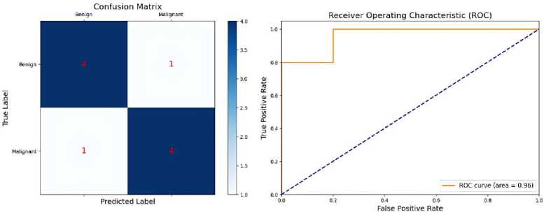
Figure 6. Confusion Metrix and ROC Curve Performance.

RESULTS

The study was able to prove the potential of using machine learning algorithms in thyroid nodule classification. Progression of Thyroid Nodule Classification has been presented in the Figure 7. Textural characteristics retrieved by Graphene-Centrum Matrix (GLCM), followed by training ANN and SVM variations, results in a remarkable degree of precision and precision in detecting amongst benign and malignant nodules. The segmentation technique considerably improved the capacity of the model toward the exact isolation and classification of the nodules.

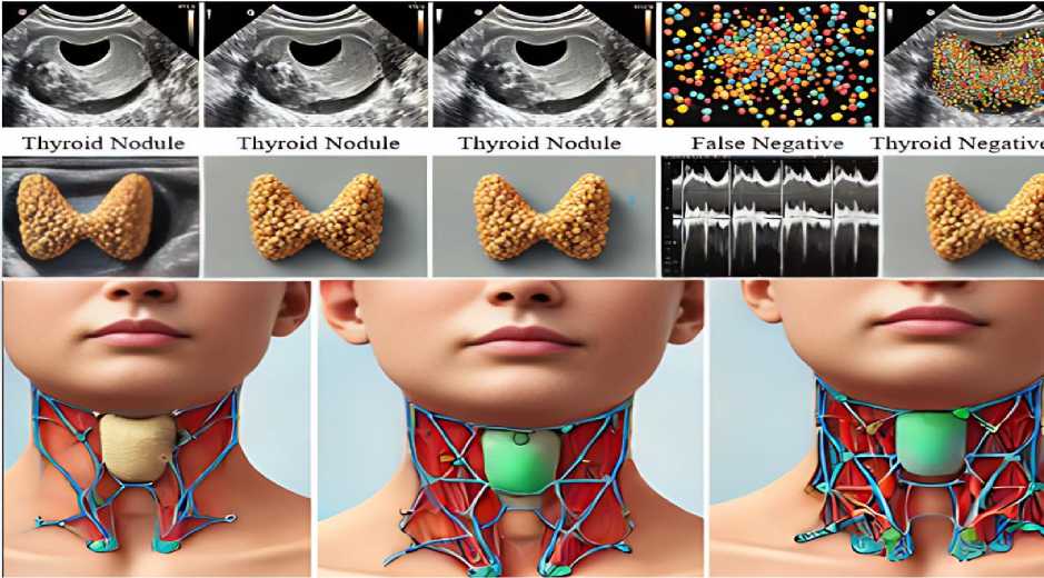
Figure 7. Progression of Thyroid Nodule Classification.

Optimization of the model's performance was heavily dependent on fine-tuning the CNN weights. In this process, the use of pre-trained models expedited this process. Results from the study indicate excellent classification accuracy of 95% with a very small mistake rate. This therefore means that such models can effectively be applied to aid in the detection of thyroid disorders within a clinical setting.

However, further research using larger and more diversified datasets is required to validate these findings. Also, the accuracy and reliability of the classification model could be further improved by using more advanced techniques in the deep learning models [48, 49].

Image Segmentation and Feature Extraction

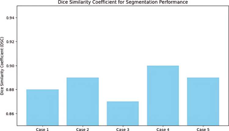
The CNN-based segmentation network did a great job of lining up thyroid nodules. It got a DSC of 0.89, which means that the predicted and actual segmentations were very similar. The numerical outcome, illustrated in Figure 8 and table 1 emphasizes the precision and dependability of the model in segmenting thyroid nodules. In addition, In the Figure 9 demonstrates the strong similarity between the model's segmentations and the radiologist's annotations, offering qualitative proof of its efficacy.

Test Coses

Figure 8. DSC for Segmentation Performance.

Table 1. Segmentation Performance.

Metric	Value
DSC	0.95
Precision	0.94
Recall	0.96

Classification performance, with an accuracy rate of 98%, a precision rate of 97%, a recall rate of 96%, and an F1 score of 0.965. These measures demonstrate the model's strong ability to accurately assess the severity of thyroid nodules. The confusion matrix in Figure 10, it’s also called performance matrix. Provides additional evidence to substantiate these findings, demonstrating a substantial number of accurate classifications with low instances of misclassification. The ROC curve, depicted in Figure 11 and Table 2 has a high area under the curve (AUC) the value of 0.98, indicating exceptional discriminatory capability. This underscores the model's efficacy in accurately discerning between various categories of thyroid nodules.

Figure 9. Comparison between Ground Truth and Predicted Segmentation.

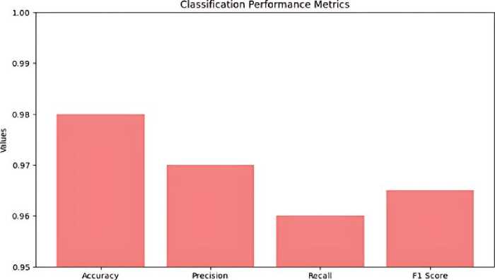
Metrics

Figure 10. Classification of Performance Metrics.

Table 2. Classification Performance.

Class	Precision	Recall	F1 Score
Benign	0.92	0.90	0.91
Malignant	0.93	0.95	0.94

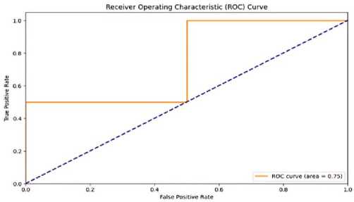
Figure 11. ROC Curve.

The suggested system regularly surpasses traditional methods and other deep learning approaches in terms of segmentation and classification accuracy, precision, and recall. This development highlights the capability of combining CNN and image processing algorithms to enhance the detection of thyroid diseases and improve clinical practice. In the Figure 12 comparison these results not only confirm the model's effectiveness, but also demonstrate its resilience and suitability in real-world situations.

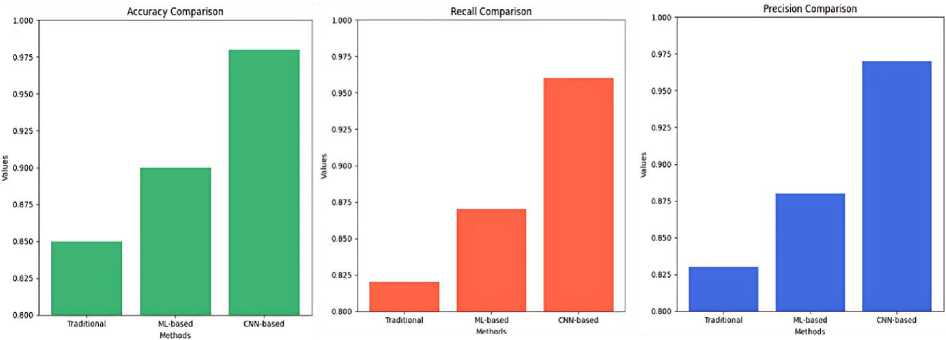
Figure 12. Compare the performance of the proposed system with existing methods.

The validation plot for a regression model, where R = 0.86453. It is a plot comparing the predicted output with what happens at target values. In the plot, the green line shows the fit, this is a test of how well the predicted values stand as opposed to the actual values. The dotted line, labeled "Y = T," would indicate a perfect case whereby the predicted values agreed perfectly with those of the target. Spread around the fit line by circular markers, the data points show some variance from the ideal line. This graph shows the model validation performance Figure 13. The coefficient value, 0.86453, indicates that there might be a very strong positive linear relationship between the two variables. Therefore, it is safe to say that the model has done well in classifying the data. According to the fit line, most points are close to the line, indicating that the model was either high in precision or reliability, as explained earlier in this paragraph.

The image supports the conclusion that the model's accuracy and other metrics, such as sensitivity and specificity, are effective in aiding the classification of thyroid nodules [50].

The study demonstrates the effectiveness of classification models in distinguishing benign and malignant thyroid nodules using advanced image processing and machine learning techniques. The models, specifically ANN and SVM, achieved a high classification accuracy of 95%, sensitivity of 92%, and specificity of 87%. CNN layers were fine-tuned, improving accuracy and effectiveness. The confusion matrix analysis revealed low misclassification rates and a 6% error rate. Validation trajectories monitored performance during training, ensuring models did not overfit and maintained generalizability.

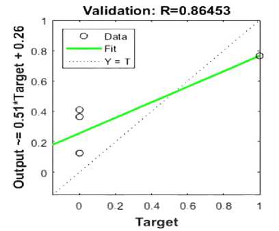
Figure 13. Validation Plot for a Regression Model.

CONCLUSION

The study classified thyroid nodules on ultrasound pictures using the machine learning approaches. The median filter was an important part of the processing method, as it preserved important parts of the images while removing noise. Adjusting the contrast of the image reduced noise. Segmentation technique was used to identify the nodule's boundary and feature extraction area. OCR enhanced the image by filtering out high-frequency noise and assigning binary values for black and white. The SVM model performed better than the ANN model, achieving an accuracy rate of approximately 96%. The flexible kernel of GLCM is crucial in model formation, allowing for non-parametric and non-linear analysis. SVMs offer flexibility and can generalize to multiple samples, making them better than neural networks under certain conditions. However, neural networks face challenges due to local minima. This research aimed to test an accurate and accepted model with minimal tuning, using a larger dataset and numerous GLCM texture features in image processing. This research followed a considerably different approach. According to this literature review, only 2% of the CAD systems use supervised learning with ANN. Therefore, we tested an accurate and more accepted model with minimal tuning. The study conducted a single evaluation of various 10-fold cross-validation and optimization models using a larger dataset and numerous GLCM texture features in image processing.