Analysis of a robust edge detection system in different color spaces using color and depth images

Determining vital parts of the digital image is a challenging area these days (especially in depth images). A lot of feature extraction methods are made and a lot of modification is applied on them so far. But extracting features in spatial and frequency domain from image, applies on whole image, even less desirable part with low amount of information. Using edge detection techniques [1], it is possible to extract just vital and highly desirable part from an image. So, after determining the vital part of the image, applying feature extraction methods is so logical. For example in extracting facial muscles features’ in facial expression recognition problem, we need to just deal with muscles part and not with other parts of the face. Using edge detection technique, it is possible to first determine and extract those muscles and then apply feature extraction algorithms on them. There are some famous traditional edge detection algorithms. Also some modified version of them is made too. Recently some other intelligent edge detection algorithms have appeared, which they use Evolutionary Algorithms (EA) [2] to determine the vital parts of the image. We are going to use the third version, which is evolutionary one, but with some modification and also some pre and post processing technique to make a bit slow but robust edge detection method. Edge detection tech- nique has application in segmentation [3] feature detection [4] object detection and tracking [5] medicine [6], biometrics [7], industry [8] and more. The paper is divided into 5 sections, which section “introduction”, defines the fundamentals needs of the problem and second section pays to some of the related research in the subject area. Section three demonstrate proposed evolutionary edge detection algorithm on different color spaces for color and depth images in details. Evaluations using benchmark test images for color and depth data, and comparing with other edge detection algorithms using Image Quality Assessment (IQA) factors in different color spaces with different noise environment is take placed in section “Validation and Results”, and final section, include the conclusion, suggestions and discussion for future works.

Color spaces

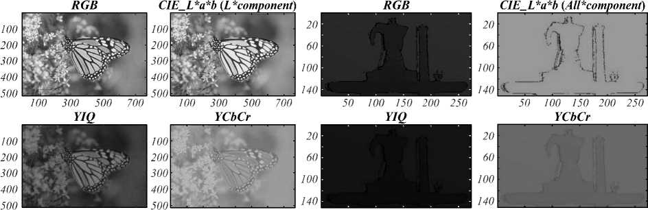
A device color space simply describes the range of colors, or gamut, that a camera can see, a printer can print, or a monitor can display. Editing color spaces, on the other hand, such as Adobe RGB or sRGB, are deviceindependent. They also determine a color range you can work in. Their design allows you to edit images in a controlled, consistent manner. A color space is a specific organization of colors. In combination with physical device profiling, it allows for reproducible representations of color, in both analog and digital representations. In order to evaluate the system we are going to use different colour space systems. Used colour spaces are RGB, CIE (Lab), YIQ and YCbCr [9– 11]. Each colour space has its characteristics. One of the most famous colour space is RGB space which is widely used by researchers and that is due to its ease of use and understanding. In Figure 1 (a), “monarch” [12– 13] benchmark test image is represented in different color space channels. Also a manually recoded depth test image (Teapot) using Kinect sensor is displayed in four color spaces in this figure too. It is mentionable that, in all tests for CIE color space, L component or channel for color data and all components or channels for depth data are used. Color spaces are represented in their actual condition, so they might not be completely visible in printed version and must be analyzed in electronic version. For example, depth data in Figure 1 (a) in YIQ and YCbCr are visible so hard for human eyes, but as this is the first step of pre-processing, could be ignored.

Figure 1 (b), represents monarch test image in different channels of CIE-Lab color space, which as it is clear, all component mode is not subtle for proposed method, which leads us to us just L channel for color data. But all channels are used for depth data. Final edge detected result is nicely visible for human eyes, as Figure 6 represents.

• 1.    RGB

• 2.    CIE 1976 or CIE (Lab)

• 3.    YIQ

• 4.    YCbCr

RGB (Red, Green and Blue) describes what kind of light needs to be emitted to produce a given color. Light is added together to create form the darkness. RGB stores individual values for red, green and blue. RGB is not a color space, it is a color model. There are many different RGB color spaces derived from this color model. The sRGB color space, or standard RGB (Red Green Blue), is an RGB color space created cooperatively by Hewlett-Packard and Microsoft Corporation for use on the Internet [9– 11].

The CIELAB color space (also known as CIE L×a×b× or sometimes abbreviated as simply "Lab" color space) is a color space defined by the International Commission on Illumination (CIE) in 1976. It expresses color as three numerical values, L× for the lightness and a× and b× for the green– red and blue–yellow color components. CIELAB was designed to be perceptually uniform with respect to human color vision. [9–11]. Also this color space is deviceindependent and includes both the gamuts of the RGB and CMYK color models.

YIQ was used in NTSC (North America, Japan and elsewhere) television broadcasts. This system stores a luma value with two chroma or chrominance values, corresponding approximately to the amounts of blue and red in the color. The Y component represents the luma information, and is the only component used by black-and-white television receivers. I and Q represent the chrominance information [9–11].

YCbCr, Y′CbCr, or Y Pb/Cb Pr/Cr, also written as YCBCR or Y'CBCR, is a family of color spaces used as a part of the color image pipeline in video and digital photography systems. Y′ is the luma component and CB and CR are the blue-difference and red-difference chroma components. Y′ (with prime) is distinguished from Y, which is luminance, meaning that light intensity is nonlinearly encoded based on gamma corrected RGB primaries [9–11].

100 300 500 700      100 300 500 700

50 100 150 200 250         50 100 150 200 250

Color

(a)

Depth

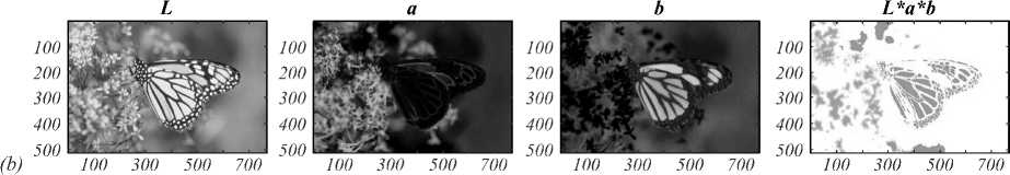
Fig. 1. (a) Monarch color test image in RGB, CIE – Lab (L component for color data and all components for depth data), YIQ and YCbCr color spaces, and manually recorded depth test image using Kinect V.2 sensor in mentioned color spaces (top). (b) Monarch test image in different L, a, b and all Lab components

Image noises

Gaussian noise is statistical noise having a probability density function (PDF) equal to that of the normal distribution, which is also known as the Gaussian distribution. The probability density function P of a Gaussian random variable Z is given by (1):

Pg (Z )=

G V2n

( Z -Ю² e ² = ²

,

where Z represents the grey level, μ the mean value and σ the standard deviation.

Principal sources of Gaussian noise in digital images arise during acquisition sensor noise caused by poor illumination and/or high temperature, and/or transmission e.g. electronic circuit noise. In digital image processing Gaussian noise can be reduced using a spatial filter, and smoothing the image with a low pass filter [14–15].

Salt-and-pepper noise (2) is a form of noise sometimes seen on images. It is also known as impulse noise. This noise can be caused by sharp and sudden disturbances in the image signal. It presents itself as sparsely occurring white and black pixels. An effective noise reduction method for this type of noise is a median filter or a morphological filter [14–15].

[ P a P ( Z M P

I 0

for z = a for z = b , otherwise

If b >  a , then gray level b will appear as a light dot in the image. If either P a or P b is zero, the impulse noise is called unipolar noise. If neither P a nor P b is zero and id they are approximately equal the impulse noise is called salt & pepper.

Shot noise or Poisson noise (3) is a type of electronic noise which can be modeled by a Poisson process. In electronics shot noise originates from the discrete nature of electric charge. Shot noise also occurs in photon counting in optical devices, where shot noise is associated with the particle nature of light [16].

N measured by a given sensor element over a time interval t is described by the discrete probability distribution

Pr (N = k ) =

e ^-X t ( X t ) ^k k !

where X is the expected number of photons per unit time interval, which is proportional to the incident scene irradiance.

Speckle noise (4) in conventional radar results from random fluctuations in the return signal from an object that is no bigger than a single image-processing element. It increases the mean grey level of a local area. The origin of this noise is seen if we model our reflectivity function as an array of scatterers. Because of the finite resolution, at any time we are receiving from a distribution of scatterers within the resolution cell.

g ( m , n ) = f ( m , n ) x u ( m , n ) x^ ( m , n ) , (4) where g (m, n) is corrupted image, u (m, n) is multiplicative component and n ( m , n ) is additive component [17].

Depth or range image and sensors

Depth or range images are type of digital images which represents the distance between object and the sensor and returns the calculated distance in different metric units depend on sensor’s type. Also this happens using different technology but mostly these sensors use infrared spectrum to capture the range. Main factor of these sensors is their vision in pure darkness like night time which is an advantage versus color sensors. Their outputs are mostly in black and white or gray scale and each pixel shows the distance till object in for example millimeter (Kinect here). Depth sensor technology is almost new but not so much and provides more information from object along with color sensor to us. Depth images are called 2.5 dimension images, because it is possible to extract 3D model of the object out of it. There are different depth sensors like Microsoft Kinect [18] Asus Xtion Pro [19] Intel® Real Sense™ Depth Camera [20] Primesense carmine [21] and more. Kinect [18] is one of the Microsoft productions for capturing color and depth images, which we used Kinect version 2 in this research (just for capturing depth data).

Prior related researches

Most of the classic edge detection operators such: Canny [22], Zerocross [23], Log [24], Roberts [25] Prewitt [26], Sobel [27] are the examples of Gradientbased edge detection methods. These operators, due to being so sensitive to noises, are not suitable for the main stage of image processing. Recently, a variety of different methods on edge detection of noisy images (without the effect of noise on the edge), has been innovated. Some of them are: wavelet transform [28], mathematical morphology method [29], neural networks [30], Fuzzy method [31] and etc. Also from evolutionary type, it is possible to refer ACO edge detection algorithm [32] or modified version of it [33]. Also a new system is made by S.M.H. Mousavi and Marwa Alkharaz in 2017 [34] which was so robust against different type of noises VS traditional edge detection algorithms.

Proposed method

The paper presents a new robust system for edge detection, which could overcome different type of noises, in different color spaces.

RGB-Gaussian (var=0.01)

100 200 300 400

CIE-Gaussian (var=0.01)

YIQ-Gaussian (var=0.01)

100 200 300 400

100 200 300 400

RGB-Poisson

100 200 300 400

CIE-Poisson

RGB-Speckle (mean=O, var=0.04)

100 200 300 400

CIE-Speckle (mean=O, var=0.04)

100 200 300 400

100 200 300 400

YIQ-Poisson

YIQ-Speckle (mean=O, var=0.04)

100 200 300 400

YCbCr-Gaussian (var=0.01)

100 200 300 400

YCbCr-Speckle (niean=O, var=0.04)

100 200 300 400

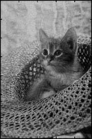
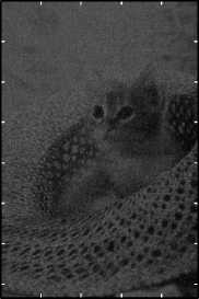
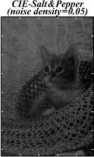
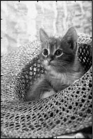
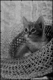
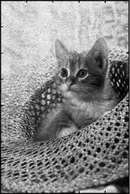
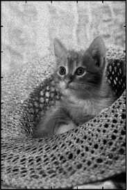
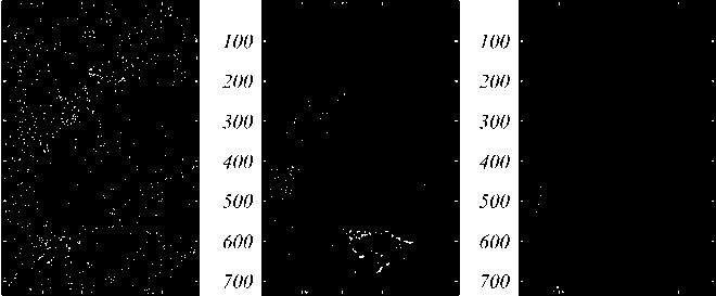
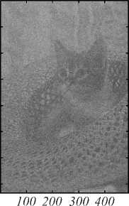
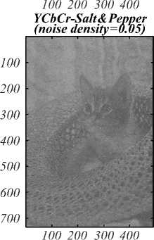
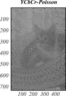
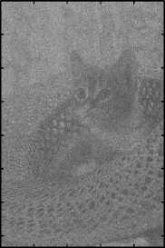
Fig. 2. Cat test image, polluted with Gaussian, Impulse, Poisson and Speckle noises in four color spaces

Filters

Our system is based on very important pre and postprocessing actions such as smoothing low pass, sharping high pass filters, morphological operations like erosion and closing, using a custom filter for evolutionary edge detection and some similar post-processing (but not all).

• 1)    Median filter

y [ m,n ] = median{ x [ i, j ] , ( i, j ) e w,

where w represents a neighborhood defined by the user, centered on location [ m , n ] in the image.

(a)

(b)

(c)

• 2)    Un-sharp masking

This technique is using to sharpening the image and effects like using high pass filter on image. Un-sharp means smooth or not sharp, and masking the un-sharp (6) is the opposite of un-sharp or not un-sharp. So it means sharp, which is applied to the edges of the image and sharp it. This technique is controlled by three main parameters which are, amount, radius and threshold. Amount is listed as a percentage and controls the magnitude of each overshoot (how much darker and how much lighter the edge borders become). Radius affects the size of the edges to be enhanced or how wide the edge rims become, so a smaller radius enhances smaller-scale detail. Threshold controls the minimal brightness change that will be sharpened or how far apart adjacent tonal values have to be before the filter does anything [43].

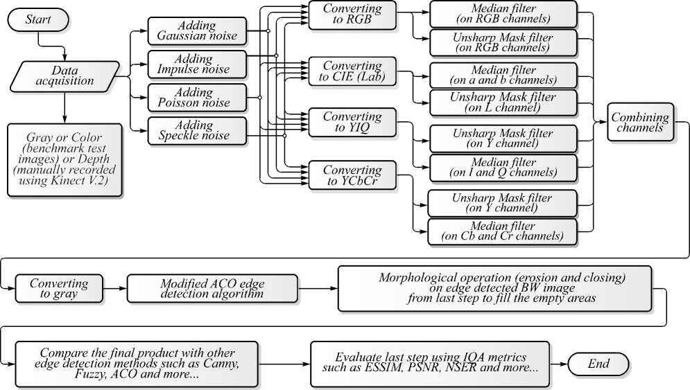
Fig. 4. Proposed method’s flowchart

Color Version

100 200 300 400 500 600 700

Depth Version

50 100 150 200 250

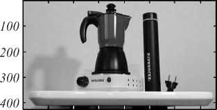
Fig. 5. Proposed method result on a manually recorded depth image using Kinect V.2 in RGB color space

Proposed Method on a Depth Version

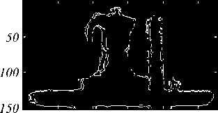
50 100 150 200 250

Un-sharp masking produce and image g ( x , y ) from an image f ( x , y ) via:

where f smooth ( x , y ) is smoother version of f ( x , y ).

Morphology operations

Morphological operators often take a binary image and a structuring element as input and combine them using a set operator (intersection, union, inclusion, complement). They process objects in the input image based on characteristics of its shape, which are encoded in the structuring element. Usually, the structuring element is sized 3×3 and has its origin at the center pixel. It is shifted over the image and at each pixel of the image its elements are compared with the set of the underlying pixels. If the two sets of elements match the condition defined by the set operator, the pixel underneath the origin of the structuring element is set to a pre-defined value (0 or 1 for binary images).

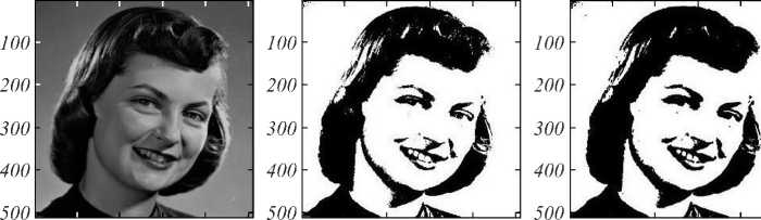
Four important morphological operation which we are going to use some of them are dilation (grow image regions), erosion (shrink image regions), opening (structured removal of image region boundary pixels) and closing (structured filling in of image region boundary pixels) [14]. For more information about morphological opera- tions, it can be referred to [14]. Figure 7 represents using these operations on “girlface” edge detected benchmark test image. We are going to use these operations for postprocessing purposes.

Let E be a Euclidean space or an integer grid, and A , a binary image in E . The erosion of the binary image A by the structuring element B is defined by (7):±

A - B = { z e E | Bz c B}, V z e E ,

where B z is the translation of B by the vector z . The erosion of A by B is also given by the (8) expression:

A - B = П A - b . beB

The dilation of A by the structuring element B is defined by (9):

A © B = U Ba. a e A

The closing of A by B is obtained by the dilation of A by B , followed by erosion of the resulting structure by B (10):

A • B = ( A © B)-B.

Modified ant colony optimization (ACO) edge detection

ACO edge detection algorithm, generate a pheromone matrix which represents edge information at each pixel position on the routes shaped by ants dispatched on the image. Ants try to find possible edges by using a heuristic information based on the degree of edginess of each pixel. The modified ACO-based edge detection [33] also uses the fuzzy clustering (FCM) to determine whether a pixel is edge or not. The algorithm is consists of three main steps of:

• •    Initialization

Artificial ants are distributed over the image, they move from one pixel to another using the transition probability which depends on local intensity.

• •    Iteratively update process

Please refer to [33].

• •    Decision process.

Pheromone matrix is used for decision making that which pixel is to be considered as edge pixel by using Ostu method of thresholding.

Figure 8 represents output of modified ACO edge detection algorithm on “MR” benchmark color test image with defined parameters in the main paper [33].

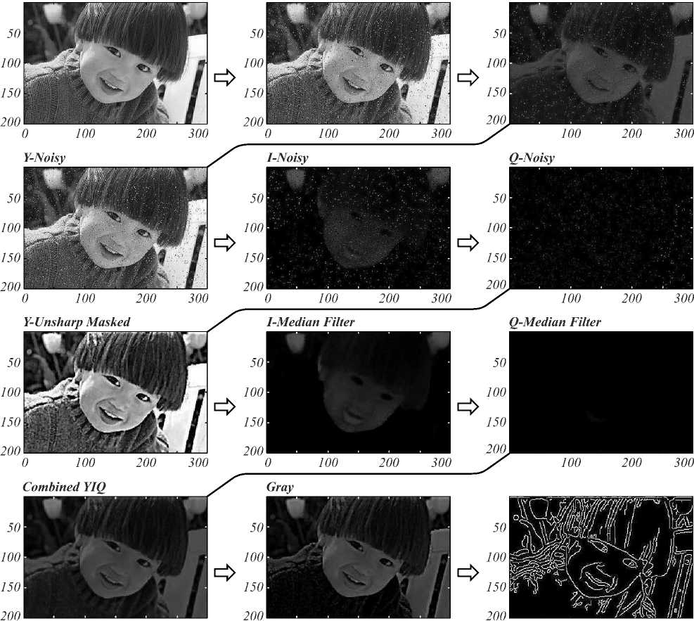
Original                              Impulse Noise-RGB                    Convert to YIQ

0       100      200    300        0       100      200     300 ________0_______ 100      200    300

[ M-ACO Edge Detection Along with Morphology )

Fig. 6. Proposed method steps on “boy” benchmark test image in YIQ color space

Original                    BW                 SE=Disk, Erode

100 200 300 400 500       100 200 300 400 500       100 200 300 400 500       100 200 300 400 500

Fig. 7. Erosion and closing morphological operations on girl face test image

SE=Disk, Closing

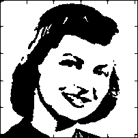
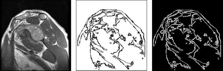
Fig. 8. Modified ACO edge detection algorithm result on MR color test image (from left to right)

Validation and results

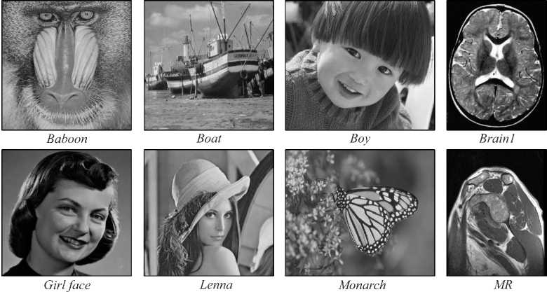
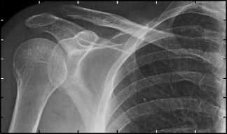
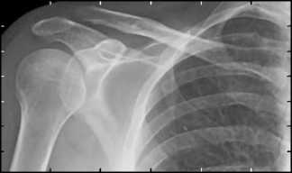
Fig. 9. 10 different color benchmark test images used for validating the proposed method

Cat

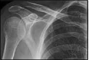
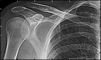
ShoulderCR

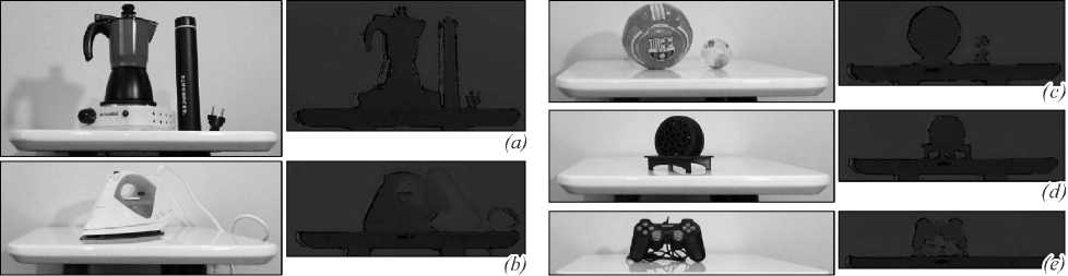
Fig. 10. 5 depth images (along with color format) which is recorded manually using Kinect V.2 sensor for validation purpose ((a) Teapot, (b) Iron, (c) Balls, (d) Coasters and (e) Joystick)

Image quality assessment factors

Image Quality Assessment ( IQA ) factors could compare the difference between two almost similar images based on images characteristics in numerical way. This similarity could be in edges, colors, brightness, shape, parts movement and more. Some of these factors which are based on edges (based on the paper subject) and some other factors will discussed for using in validation section.

ESSIM =

= function ( l , ( 1 1 , 1 2 ) , c ( 1 1 , 1 2 ) , e ( 1 1 , 1 2 ) ) ..

It is the edge oriented version of SSIM metric [44].The following steps do the computation of this metric:

• •    Vertical and Horizontal maps are created by the use of Sobel operator.

• •    Image is sub-sampled to 16 x 16 blocks.

• •    Histogram of edge direction is created according to the sum of amplitudes with similar (1/8) directions.

• •    Using standard deviations of obtained histograms the edge factor is calculated in (12).

e ( I„ 1 2 ) = °^Ш 2 + C 3

° 1 1 ^CT 1 2 + C 3

.

Application of Sobel filter is considered to be time efficient, effective and simple. Provides better performance than PSNR and SSIM in evaluation and had a good response to image degradation.

It indicates the level of losses or signals integrity. The Peak Signal to Noise Ratio ( PSNR ) (13) block computes the peak signal-to-noise ratio, in decibels, between two images. This ratio is often used as a quality measurement between the original and a compressed image. The higher the PSNR , the better the quality of the compressed, or reconstructed image [36].

PSNR = 10 log.,,-----

¹⁰ MSE

in which L determines the range of value, which a pixel could have. Its unit is DB, and has a limit of 50. The proper value is between 20 and 50.

The Mean Square Error ( MSE ) (14) and the Peak Signal to Noise Ratio ( PSNR ) are the two error metrics used to compare image compression quality. The MSE represents the cumulative squared error between the compressed and the original image, whereas PSNR represents a measure of the peak error. The lower the value of MSE , the lower the error [37].

N -1 M -1

ME=77-7 SD X M-Y (i-j )]2.

M ^{x N} i =0 j =0

In which, X and Y are two arrays with the size of M x N . To any extent Y resembles X , the value of MSE will reduce.

4) EME ( Enhancement Measure )

Measure of enhancement (15) is another image quality metric or assessment. This measure is related with concepts of the Webers Low of the human visual system. It helps to choose (automatically) the best parameters and transform [38].

EME = max

Фе { ф }

%( EME (Ф)),

which max = Фе { ф }

%

k2 k1              T го zi20log I-max^

^k 1 k 2 l =1 k =1            I min ; k ; l

Let an image x ( n , m ) be splitted into k 1 k 2 blocks w k ,l ( i , j ) of size l 1 x 1 ₂ and let { Ф } to be a given class of orthogonal transform used for image enhancement. Also r ^ ax ; k ; 1 and I “ _{n ; k ;} l are respectively minimum and maximum of the image x ( m , m ) inside the block w k ,l. The function % is the sign function.

• 5)    Edge Based Image Quality Assessment ( EBIQA )

Edge preservation one of the most important aspect during the human visual assessment. Attar, Shahbahrami, and Rad proposed Edge Based Image Quality Assessment (EBIQA) technique that aims to operate on the human perception of the features [39]. Steps are:

• •    Edges locations are identified utilizing Sobel edge detector technique in both images.

• •    The 16x16 pixel window size vectors are formed at each image based on (16) and (17), -where I 1 is reference image and I 2 is the image under test.

1 1 = ( O , AL , PL , N , VHO ) ,

12 = ( O , AL , PL , N , VHO ) ,                      (17)

which ’ O ’ stands for edge orientation in the image, which is a total number of edges. ’ AL ’ or value of the average length of all edges. ’ PL ’ estimates the number of pixels with a similar level of intensity values. ’ N ’ responds for sum of pixels, which form edges. ’ VH ’ corresponds for sum of pixels, which form edges in either vertically or horizontally located edges. Finally, we estimate EBIQA by (18), where average Euclidean distance of proposed vectors is estimated.

MN

EBIQA = ZZ ( I i - I 2 ) 2 .                (18)

MN / =1 j =i

• 6)    Non-Shift Edge Based Ratio ( NSER )

This method is based on zero-crossings and was proposed by Zhang, Mou and Zhang [40]. It makes decisions upon edge maps. Steps are as follow:

• •    Gaussian kernel is applied to the interesting images on different standard deviation scales to identify edges.

• •    Then operation is performed between two images. Ratio of the common edge number located by initial edge number is found using (19):

A =| I 1 ^ 1 2IH I JI-                               (19)

The result of this operation is normalized by log function to improve correlation factor (20):

N

NSER ( 1 1 , 1 2 ) = - £ log10 ( 1 - p , ) .               (20)

i =1

• 7)    Gradient Conduction Mean Square Error ( GCM-SE )

Lopez-Randulfe et al. in their paper introduced an edge aware metric based on MSE [37]. In this algorithm weighted sum of gradients (distance pixels) is taken into account [41]. GCMSE Provides better performance than MSE and SSIM . The main steps are as follow:

• • Directional gradients are estimated in four directions using (21) and then average value G p is found. Note that the results are optimized by the coefficient k:

G = ( 1 2 - 1 1 )²

( 1 2 — 1 1 )² + k ^2.

The GCMSE is estimated based on (22):

GCMSE =

z : =1 Z n = =д 1 2 ( x , y ) - 1 1 ( x , y ) ) G p ] 2

C 1 + Z m Z n G

L-i x=1L^ y =1 ^p

. (22)

Validation’s results

As we have 7 IQA metrics, 15 color and depth test images, 9 comparing methods, 4 noise types and 4 color spaces, representing this amount of combinations in table format requires 112 (15x11) tables which is not possible to fit in the paper. Due to that, we decided to select 7 tables which covers all areas of changes and results from these 112 tables. But as we analyzed the results, proposed method was so robust versus other methods, as some of these results are represented in Tables 1 –7. Also we selected 7 table which covers all 7 IQA metrics with (diverse noise and color spaces). Comparisons are based on un-noised edge detected versions on the test images versus noisy versions using IQA metrics. For example and for baboon test image in CIE color space with Gaussian noise, calculated with ESSIM IQA metric, edge detection using Sobel operators performs and the acquired image is going to compare with un-noised version of the baboon test image. This happens for all edge detection methods in same condition on same test image. Then it is possible to compare acquired results in bigger view on tables.

Note that all the comparing results are normalized between 0-1 ranges for better understanding (even PSNR).

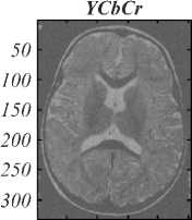
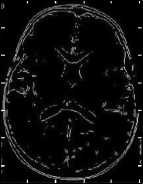
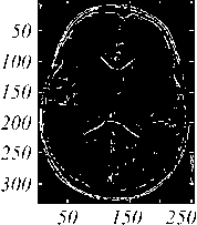
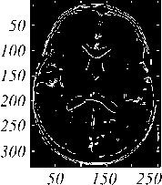
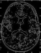
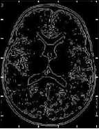
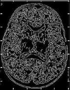
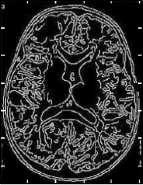
As the result are closer to 1, it shows better results or highest similarity (depend on the metric’s definition) and vice versa. Tables 1 to 7 represent evaluations results from 7 IQA metrics for comparing different edge detection methods (including proposed method) on diverse test images (color and depth) using ESSIM, PSNR, MSE, EME, EBIQA, NSER and GCMSE metrics, respectively with different noises and in different color spaces. Figure 11 shows the visual comparison between proposed method and other methods in YCbCr color space which Brain1 test image is polluted with Speckle noise. It is mentionable that lower and upper threshold value for canny edge detector was [0.01, 0.12]. As it is clear in Figure 11, a lot of details are presented on each method, due to brain’s structure and lines. So it might not be analyzable in printed version and should be used electronic version of the image for full details. After making different types of edge detection techniques in decades by other researchers, now it is time to pay to the details after all to make a promising new method.

Conclusion discussion and suggestions

With using evolutionary algorithm, it is possible to achieve proper result in edge detection subject, just like other subjects in artifactual intelligence. It is concluded that, different color spaces have different effects on different edge detection methods and different results could be acquired. But with a precise look at the results, we can see that RGB and YIQ are the best color spaces for edge detection. Also YCbCr color space is not so bad, but CIE color space is better for depth data than color. Proposed evolutionary edge detection had perfect robustness against Impulse and Poisson noises in different color spaces. Speckle and Gaussian noises are in next ranks in relation to robustness. Validation results represents that proposed method returned more results close to 1 versus other methods for IQA metrics, which this shows the power of proposed method in different conditions. In the other hand, proposed method returned promising and satisfactory results on manually recorded depth images with Kinect V.2 that could open ways in this era too. Also system is almost fast and can work in real time purposes too. It is suggested to use other evolutionary algorithms for edge detection purposes such as ABC [45], Bat algorithm [46], PSO [47], GGO [48] and ICA [49], which may perform better in that way.

Sobel

50   150 250

Roberts

Prewitt

50 100 150 200 250 300

50   150 250

Log

Zerocross

50   150 250

Canny

50   150 250

Proposed Method

50 150 250

50   150 250

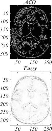
Fig. 11. The visual comparison between proposed method and other methods in YCbCr color space which Brain1 test image is polluted with Speckle noise

Table 1. Comparing various methods with ESSIM (Impulse noise in YIQ color space)

	Test Images	Sobel	Roberts	Prewitt	Log	Cross	Canny	[34]	ACO	Proposed	Fuzzy
Color
1	baboon	0.623	0.614	0.523	0.762	0.715	0.786	0.803	0.802	0.811	0.762
2	boat	0.515	0.504	0.413	0.652	0.605	0.676	0.693	0.696	0.701	0.652
3	boy	0.748	0.736	0.645	0.884	0.837	0.908	0.925	0.924	0.933	0.884
4	Brain1	0.701	0.694	0.603	0.842	0.795	0.866	0.883	0.882	0.897	0.842
5	cat	0.592	0.588	0.497	0.736	0.689	0.760	0.777	0.776	0.785	0.736
6	girl face	0.681	0.679	0.588	0.827	0.780	0.851	0.898	0.865	0.896	0.827
7	Lenna	0.622	0.615	0.524	0.763	0.716	0.787	0.804	0.803	0.812	0.763
8	monarch	0.724	0.714	0.623	0.862	0.815	0.886	0.903	0.904	0.911	0.862
9	MR	0.773	0.762	0.671	0.910	0.863	0.934	0.951	0.950	0.959	0.910
10	shoulderCR	0.574	0.561	0.470	0.709	0.662	0.733	0.750	0.749	0.758	0.709
Depth
11	Balls	0.668	0.658	0.567	0.806	0.759	0.830	0.847	0.843	0.855	0.806
12	Coasters	0.627	0.619	0.528	0.767	0.720	0.791	0.808	0.807	0.816	0.767
13	Iron	0.697	0.681	0.590	0.829	0.782	0.853	0.870	0.862	0.878	0.829
14	Joystick	0.605	0.596	0.505	0.744	0.697	0.768	0.785	0.784	0.793	0.744
15	Teapot	0.718	0.704	0.613	0.852	0.805	0.876	0.893	0.891	0.901	0.852

Table 2. Comparing various methods with PSNR (Poisson noise in RGB color space)

	Test Images	Sobel	Roberts	Prewitt	Log	Cross	Canny	[34]	ACO	Proposed	Fuzzy
Color
1	baboon	0.574	0.702	0.730	0.768	0.761	0.902	0.920	0.919	0.921	0.876
2	boat	0.454	0.582	0.610	0.648	0.642	0.782	0.800	0.799	0.801	0.756
3	boy	0.633	0.761	0.789	0.827	0.822	0.961	0.979	0.978	0.980	0.935
4	Brain1	0.548	0.676	0.704	0.742	0.734	0.876	0.904	0.893	0.895	0.850
5	cat	0.538	0.666	0.694	0.732	0.726	0.866	0.884	0.883	0.885	0.840
6	girl face	0.543	0.671	0.699	0.737	0.735	0.871	0.889	0.888	0.890	0.845
7	Lenna	0.565	0.693	0.721	0.759	0.753	0.893	0.911	0.910	0.912	0.867
8	monarch	0.625	0.753	0.781	0.819	0.816	0.953	0.971	0.970	0.972	0.927
9	MR	0.640	0.768	0.796	0.834	0.828	0.968	0.986	0.985	0.987	0.942
10	shoulderCR	0.511	0.639	0.667	0.705	0.697	0.839	0.857	0.856	0.858	0.813
Depth
11	Balls	0.526	0.654	0.682	0.720	0.718	0.854	0.872	0.871	0.873	0.828
12	Coasters	0.550	0.678	0.706	0.744	0.738	0.878	0.896	0.895	0.897	0.852
13	Iron	0.571	0.699	0.727	0.765	0.758	0.899	0.917	0.916	0.918	0.873
14	Joystick	0.506	0.634	0.662	0.700	0.699	0.834	0.852	0.851	0.853	0.808
15	Teapot	0.589	0.717	0.745	0.783	0.770	0.917	0.935	0.934	0.936	0.893

Table 3. Comparing various methods with MSE (Gaussian noise in CIE color space)

	Test Images	Sobel	Roberts	Prewitt	Log	Cross	Canny	[34]	ACO	Proposed	Fuzzy
Color
1	baboon	0.568	0.594	0.604	0.722	0.653	0.730	0.731	0.700	0.746	0.726
2	boat	0.548	0.574	0.580	0.702	0.633	0.710	0.711	0.680	0.723	0.706
3	boy	0.712	0.638	0.641	0.866	0.797	0.874	0.875	0.844	0.890	0.870
4	Brain1	0.649	0.575	0.583	0.803	0.734	0.811	0.812	0.781	0.827	0.807
5	cat	0.560	0.586	0.592	0.714	0.645	0.722	0.723	0.692	0.738	0.718
6	girl face	0.659	0.585	0.593	0.813	0.744	0.821	0.822	0.791	0.844	0.825
7	Lenna	0.560	0.586	0.594	0.714	0.645	0.722	0.723	0.692	0.738	0.718
8	monarch	0.696	0.622	0.635	0.750	0.781	0.898	0.859	0.828	0.874	0.891
9	MR	0.708	0.634	0.642	0.762	0.793	0.870	0.871	0.840	0.926	0.876
10	shoulderCR	0.574	0.593	0.606	0.721	0.652	0.729	0.730	0.699	0.743	0.725
Depth
11	Balls	0.566	0.592	0.601	0.720	0.651	0.728	0.729	0.698	0.743	0.724
12	Coasters	0.565	0.591	0.600	0.719	0.650	0.727	0.728	0.697	0.739	0.723
13	Iron	0.708	0.553	0.561	0.781	0.712	0.889	0.890	0.759	0.895	0.785
14	Joystick	0.574	0.600	0.610	0.728	0.659	0.736	0.737	0.706	0.750	0.733
15	Teapot	0.559	0.583	0.591	0.711	0.642	0.719	0.720	0.689	0.730	0.715

Table 4. Comparing various methods with EME (Speckle noise in YCbCr color space)

	Test Images	Sobel	Roberts	Prewitt	Log	Cross	Canny	[34]	ACO	Proposed	Fuzzy
Color
1	baboon	0.603	0.517	0.455	0.803	0.715	0.828	0.817	0.816	0.829	0.814
2	boat	0.505	0.419	0.357	0.705	0.617	0.730	0.705	0.718	0.731	0.716
3	boy	0.704	0.618	0.556	0.904	0.816	0.929	0.928	0.917	0.930	0.915
4	Brain1	0.625	0.539	0.477	0.825	0.737	0.85	0.894	0.838	0.901	0.836
5	cat	0.509	0.423	0.361	0.709	0.621	0.734	0.713	0.722	0.735	0.720
6	girl face	0.590	0.504	0.442	0.790	0.702	0.815	0.807	0.803	0.816	0.801
7	Lenna	0.584	0.498	0.436	0.784	0.696	0.809	0.782	0.797	0.810	0.795
8	monarch	0.655	0.569	0.507	0.855	0.767	0.880	0.858	0.868	0.881	0.866
9	MR	0.673	0.587	0.525	0.873	0.785	0.898	0.872	0.886	0.890	0.884
10	shoulderCR	0.512	0.426	0.364	0.712	0.624	0.737	0.718	0.725	0.738	0.723
Depth
11	Balls	0.589	0.503	0.441	0.789	0.701	0.814	0.793	0.802	0.815	0.800
12	Coasters	0.550	0.464	0.402	0.750	0.662	0.775	0.753	0.762	0.776	0.761
13	Iron	0.612	0.526	0.464	0.812	0.724	0.837	0.813	0.825	0.838	0.823
14	Joystick	0.537	0.451	0.389	0.737	0.649	0.762	0.760	0.750	0.763	0.748
15	Teapot	0.582	0.496	0.434	0.782	0.694	0.807	0.782	0.741	0.808	0.793

Table 5. Comparing various methods with EBIQA (Impulse noise in CIE color space)

	Test Images	Sobel	Roberts	Prewitt	Log	Cross	Canny	[34]	ACO	Proposed	Fuzzy
Color
1	baboon	0.567	0.602	0.616	0.577	0.569	0.642	0.725	0.724	0.732	0.664
2	boat	0.617	0.552	0.565	0.627	0.619	0.593	0.675	0.643	0.682	0.644
3	boy	0.629	0.564	0.674	0.910	0.794	0.807	0.921	0.893	0.924	0.886
4	Brain1	0.537	0.572	0.585	0.647	0.639	0.715	0.795	0.762	0.882	0.744
5	cat	0.583	0.616	0.574	0.591	0.583	0.655	0.739	0.706	0.746	0.738
6	girl face	0.538	0.573	0.585	0.648	0.640	0.716	0.796	0.764	0.803	0.745
7	Lenna	0.598	0.533	0.548	0.608	0.600	0.676	0.756	0.730	0.763	0.655
8	monarch	0.583	0.618	0.633	0.693	0.685	0.898	0.879	0.806	0.898	0.888
9	MR	0.595	0.630	0.648	0.705	0.697	0.773	0.853	0.816	0.880	0.892
10	shoulderCR	0.597	0.532	0.549	0.607	0.599	0.678	0.755	0.722	0.762	0.654
Depth
11	Balls	0.624	0.559	0.574	0.634	0.626	0.709	0.782	0.749	0.789	0.790
12	Coasters	0.602	0.537	0.557	0.612	0.604	0.680	0.760	0.726	0.767	0.759
13	Iron	0.580	0.615	0.630	0.590	0.582	0.660	0.738	0.705	0.745	0.637
14	Joystick	0.599	0.534	0.546	0.609	0.608	0.680	0.757	0.726	0.764	0.656
15	Teapot	0.627	0.562	0.677	0.907	0.899	0.801	0.895	0.897	0.924	0.894

Table 6. Comparing various methods with NSER (Poisson noise in YIQ color space)

	Test Images	Sobel	Roberts	Prewitt	Log	Cross	Canny	[34]	ACO	Proposed	Fuzzy
Color
1	baboon	0.513	0.496	0.678	0.773	0.806	0.837	0.859	0.843	0.874	0.796
2	boat	0.450	0.433	0.615	0.718	0.743	0.774	0.796	0.78	0.811	0.733
3	boy	0.558	0.541	0.723	0.827	0.851	0.882	0.904	0.888	0.919	0.841
4	Brain1	0.535	0.518	0.700	0.798	0.828	0.859	0.881	0.865	0.896	0.818
5	cat	0.423	0.406	0.588	0.687	0.716	0.747	0.769	0.753	0.784	0.706
6	girl face	0.506	0.489	0.671	0.769	0.799	0.83	0.852	0.836	0.867	0.789
7	Lenna	0.474	0.457	0.639	0.738	0.767	0.798	0.82	0.804	0.835	0.757
8	monarch	0.567	0.550	0.732	0.880	0.860	0.891	0.913	0.897	0.928	0.850
9	MR	0.539	0.522	0.704	0.802	0.832	0.863	0.885	0.869	0.900	0.822
10	shoulderCR	0.340	0.323	0.505	0.609	0.633	0.664	0.686	0.670	0.701	0.623
Depth
11	Balls	0.455	0.438	0.62	0.715	0.748	0.779	0.801	0.785	0.816	0.738
12	Coasters	0.464	0.447	0.629	0.722	0.757	0.788	0.81	0.794	0.825	0.747
13	Iron	0.478	0.461	0.643	0.741	0.771	0.802	0.824	0.808	0.839	0.761
14	Joystick	0.424	0.407	0.589	0.683	0.717	0.748	0.77	0.754	0.785	0.707
15	Teapot	0.561	0.544	0.726	0.823	0.854	0.895	0.907	0.891	0.922	0.844

Table 7. Comparing various methods with GCMSE (Speckle noise in YCbCr color space)

	Test Images	Sobel	Roberts	Prewitt	Log	Cross	Canny	[34]	ACO	Proposed	Fuzzy
Color
1	baboon	0.556	0.521	0.488	0.659	0.691	0.726	0.719	0.764	0.786	0.751
2	boat	0.443	0.411	0.378	0.545	0.581	0.616	0.609	0.654	0.673	0.641
3	boy	0.623	0.593	0.56	0.723	0.763	0.798	0.791	0.836	0.853	0.823
4	Brain1	0.613	0.581	0.548	0.716	0.751	0.786	0.879	0.824	0.896	0.811
5	cat	0.395	0.365	0.332	0.496	0.535	0.570	0.563	0.608	0.724	0.595
6	girl face	0.633	0.606	0.573	0.736	0.776	0.811	0.804	0.849	0.866	0.836
7	Lenna	0.576	0.542	0.509	0.677	0.712	0.747	0.740	0.785	0.805	0.772
8	monarch	0.579	0.549	0.516	0.679	0.719	0.754	0.747	0.792	0.803	0.779
9	MR	0.709	0.673	0.640	0.804	0.843	0.878	0.897	0.916	0.933	0.903
10	shoulderCR	0.508	0.478	0.445	0.604	0.648	0.683	0.676	0.721	0.736	0.708
Depth
11	Balls	0.550	0.525	0.492	0.654	0.695	0.730	0.723	0.768	0.785	0.755
12	Coasters	0.530	0.506	0.473	0.634	0.676	0.711	0.704	0.749	0.766	0.736
13	Iron	0.617	0.588	0.555	0.718	0.758	0.793	0.786	0.831	0.847	0.818
14	Joystick	0.618	0.583	0.55	0.719	0.753	0.788	0.781	0.826	0.898	0.813
15	Teapot	0.658	0.628	0.595	0.759	0.798	0.833	0.896	0.871	0.899	0.858

• [17]    Jaybhay J, Shastri R. A study of speckle noise reduction filters. Signal & Image Processing: An International Journal (SIPIJ) 2015; 6.

• [18]    Zhang Zh. Microsoft kinect sensor and its effect. IEEE Multimedia 2012; 19(2): 4-10.

• [19]    Xtion PRO. Source:     〈 https://www.asus.com/3D-

• Sensor/Xtion_PRO/〉.

• [20]    Keselman L, et al. Intel RealSense stereoscopic depthcameras. Source: 〈 https://arxiv.org/abs/1705.05548〉 .

• [21]    Primesense Carmine 1.09. Source: 〈 http://xtionprolive.com/primesense-carmine-1.09〉 .

• [22]    Canny J. A computational approach to edge detection. In Book: Fischler MA, Firschein O, eds. Readings in computer vision: issues, problems, principles, and paradigms. San Francisco, CA: Morgan Kaufmann Publishers Inc; 1987: 184-203.

• [23]    Haralick RM. Digital step edges from zero crossing of second directional derivatives. IEEE Transactions on Pattern Analysis and Machine Intelligence 1984; 1: 58-68.

• [24]    Lindeberg T. Scale selection properties of generalized scale-space interest point detectors. Journal of Mathematical Imaging and Vision 2013; 46(2): 177-210.

• [25]    Roberts LG. Machine perception of three-dimensional solids. Diss PhD Thesis. Cambridge, MA; 1963.

• [26]    Prewitt JMS. Object enhancement and extraction. Picture Processing and Psychopictorics 1970; 10(1): 15-19.

• [27]    Sobel I, Feldman G. A 3x3 isotropic gradient operator for image processing, presented at a talk at the Stanford Artificial Project. In Book: Duda R, Hart P, eds. Pattern classification and scene analysis. John Wiley & Sons; 1968: 271-272.

• [28]    Shih M-Y, Tseng D-Ch. A wavelet-based multiresolution edge detection and tracking. Image and Vision Computing 2005; 23(4): 441-451.

• [29]    Lee J, Haralick R, Shapiro L. Morphologic edge detection. IEEE Journal on Robotics and Automation 1987; 3(2): 142-156.

• [30]    Rajab, MI, Woolfson MS, Morgan SP. Application of region-based segmentation and neural network edge detection to skin lesions. Computerized Medical Imaging and Graphics 2004; 28(1): 61-68.

• [31]    Akbari AS, Soraghan JJ. Fuzzy-based multiscale edge detection. Electronics Letters 2003; 39(1): 30-32.

• [32]    Tian J, Yu W, Xie S. An ant colony optimization algorithm for image edge detection. 2008 IEEE Congress on Evolutionary Computation (IEEE World Congress on Computational Intelligence) 2008: 751-756.

• [33]    Rajeswari R, Rajesh R. A modified ant colony optimization based approach for image edge detection. 2011 International Conference on Image Information Processing, 2011.

• [34]    Mousavi SMH, Kharazi M. An edge detection system for polluted images by gaussian, salt and pepper, poisson and speckle noises. 4^th National Conference on Information Technology, Computer & TeleCommunication 2017.

• [35]    Chen G-H, et al. Edge-based structural similarity for image quality assessment. 2006 IEEE International Conference on Acoustics Speech and Signal Processing 2006; 2: II-II.

• [36]    Wang Z, et al. Image quality assessment: from error visibility to structural similarity. IEEE Transactions on Image Processing 2004; 13(4): 600-612.

• [37]    Lehmann EL, Casella G. Theory of point estimation. Springer Science & Business Media; 2006.

• [38]    Agaian SS, Lentz KP, Grigoryan AM. A new measure of image enhancement. IASTED International Conference on Signal Processing & Communication 2000.

• [39]    Attar A, Shahbahrami A, Rad RM. Image quality assessment using edge based features. Multimedia Tools and Applications 2016; 75(12): 7407-7422.

• [40]    Zhang M, Mou X, Zhang L. Non-shift edge based ratio (NSER): An image quality assessment metric based on early vision features. IEEE Signal Processing Letters 2011; 18(5): 315-318.

• [41]    López-Randulfe J, et al. A quantitative method for selecting denoising filters, based on a new edge-sensitive metric. 2017 IEEE International Conference on Industrial Technology (ICIT) 2017: 974-979.

• [42]    Huang T, Yang G, Tang G. A fast two-dimensional median filtering algorithm. IEEE Transactions on Acoustics, Speech, and Signal Processing 1979; 27(1): 13-18.

• [43]    Polesel A, Ramponi G, Mathews VJ. Image enhancement via adaptive unsharp masking. IEEE Transactions on Image Processing 2000; 9(3): 505-510.

• [44]    Wang Z, et al. Image quality assessment: from error visibility to structural similarity. IEEE Transactions on Image Processing 2004; 13(4): 600-612.

• [45]    Karaboga D. An idea based on honey bee swarm for numerical optimization. Technical Report-TR06. Erciyes University, Turkey; 2005.

• [46]    Yang X-S. A new metaheuristic bat-inspired algorithm. In Book: González JR, Pelta DA, Cruz C, Terrazas G, Kras-nogor N, eds. Nature inspired cooperative strategies for optimization (NICSO 2010). Berlin, Heidelberg: Springer; 2010: 65-74.

• [47]    Kennedy J. Particle swarm optimization. In Book: Sammut C, Webb GI, eds. Encyclopedia of Machine Learning. Boston, MA: Springer US; 2011: 760-766.

• [48]    Hossein Mousavi SM, Mirinezhad SY, Dezfoulian MH. Galaxy gravity optimization (GGO) an algorithm for optimization, inspired by comets life cycle. 2017 Artificial Intelligence and Signal Processing Conference (AISP) 2017: 306-315.

• [49]    Atashpaz-Gargari E, Lucas C. Imperialist competitive algorithm: an algorithm for optimization inspired by imperialistic competition. 2007 IEEE Congress on Evolutionary Computation 2007: 4661-4667.