Analysis of Reconfigurable Processors Using Petri Net

Published Online July 2013 in MECS (http://www.

Reconfigurable computing has proven to be promising technology to increase the performance of certain algorithms in scientfiic and engineering applications in recent years. Any application of iterative nature such as image processing, digital signal processing, bioinformatics, cryptography and software dfiened radio etc; can be mapped on an FPGA by programming it with Hardware Descriptive Languages (HDLs). These applications have certain kernels containing interactions which are processed in parallel on the processing elements on an FPGA dfiened by the HDL programmer. The same applications can take much longer time, when they are run on a General Purpose Processor (GPP) which processes the iterative kernels in a sequential manner. Traditionally, the grids utilize GPPs as their main processing elements. Because of incorporation of the REs in the grid network, there is need for appropriate models for these new processing elements to investigate the possibility of their utilization for compute intensive kernels of the grid applications. Many grid networks, such as TeraGrid are incorporating figreucroanble computing resources in addition to general-purpose processors (GPPs) as processing elements and this combination offers better performance and higher flexibility. An approach to achieve high-performance with flexibility is to utilize collaboration of reconfigurable computing elements in grid networks.

Petri nets (PNs) provide a graphical tool as well as a notational method for the formal specification of systems. Petri nets were first introduced in 1966 to describe concurrent systems. Every tool applied to the modeling and analysis of computer systems has its place. Several design methodologies for embedded systems based on different formal models have been developed in recent years. Example is the project Moses [1], which is based on high level Petri nets. Many processes may be described as a logical sequence of events. This has led the authors, among others, to the development and use of Petri nets as a tool for process and condition monitoring (PCM) [2-5]. Petri net provides powerful qualitative analysis and quantitive analysis for specifying behavior and an executable notation. Petri net have a place in computer systems performance assessment, ranging somewhere between analytical queuing theory and computer simulation. This is due to the nature of Petri nets and their ability to model concurrency, synchronization, mutual exclusion, conflict, and systems state more completely than analytical models but not as completely as simulations. Petri nets represent computer systems by providing a mean to abstract the basic elements of the system and its informational flow using only four fundamental components.

Reconfigurable computing is turning into a suitable technology for high-performance computing in scientific research. An appropriate Petri net model for reconfigurable elements along with general purpose processors is essential for analytical performance modeling of an application. There is need for promising models for new processing elements to investigate the possibility of their utilization for computing intensive kernels of the applications. The results of simulations can help in designing a system by saving a significant amount of time and resources.

In this work, the development of a model, based on the Petri net is proposed, we proposed theoretical model for processors using Petri net. We simulated the proposed models as part of a large network. The simulation results suggest that the total average error rate for all models is less than 5%, also the analysis time in these models is 0.016 seconds.

The remainder of the paper is organized as follows: Section II presents related research. Section III introduces the related terminology. In section IV the proposed models for processing components are presented. Section V shows the simulation results. Finally, the conclusion is provided in Section VI.

• II.    RELATED WORKS

In this section, we discuss some related work for the modeling and simulation of reconfigurable processors.

In [6] an analytical model was proposed for reconfigurable processors using the queuing theory. The results show that the main limitation of such a system is the reconfigurable time. The model, however, does not take into account the modeling of memory modules which must be considered in real scenarios. Some developed abstract model for a reconfigurable computer, [7] focused on the performance model for runtime reconfigurable hardware accelerators. In a theoretical analysis, the factors such as speedup, communication and configuration overheads are considered, but this model does not consider the utilization of the accelerator in a network perspective. In [8] was proposed an abstract model for a reconfigurable computer which utilized both the GPP and the RE. In [9] a modeling for multiprocessor system using Petri net proposed, and [10] focused a model for a system using generalized stochastic Petri nets.

• III.    DEFINITION AND CONCEPTS

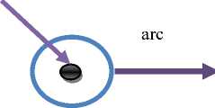
Petri net components are place, transition, arcs, and token. Places are represented graphically as a circle, transitions as a bar, arcs as directed line segments, and tokens as dots (Figure 1). Places are used to represent possible system components and their state. For example, a disk drive could be represented using a place, as could a program or other resource. Transitions are used to describe events that may result in different system states. For example, the action of reading an item from a disk drive or the action of writing an item to a disk drive could be modeled as separate transitions. Arcs represent the relationships that exist between the transitions and places. For example, disk read requests may be put in one place, and that place may be connected to the transition, removing an item from a disk thus indicating that this place is related to the transition.

Arcs provide a path for the activation of a transition; tokens are used to define the state of the Petri net. Tokens in the basic Petri net model are non-descriptive markers, which are stored in places and are used in defining Petri net marking [11].

Token

Place p

Transition t

Figure 1 : Basic Petri net Component

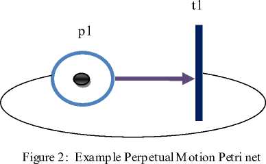
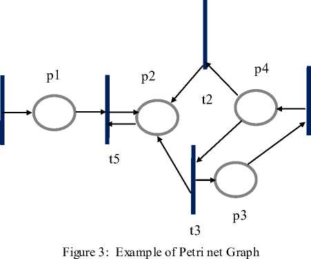
The marking of a Petri net place by the placement of a token can be viewed as the statement of the condition of the place. For example, a simple Petri net with only one place and one transition is depicted in the Figure 2. The place is connected to the transition by an arc, and the transition is likewise connected to the place by a second arc. The former arc is an input arc, while the latter arc is an output arc. The placement of a token represents the active marking of the Petri net state. The Petri net shown in Figure 2 represents a net that will continue to cycle forever. A Petri net is shown as a five tuple, M = (P, T, I, O, MP), where P portrays a set of places, P = {p1, p2,…, pn}, with one place for each circle in the Petri net graph; T portrays a set of transitions, T = {t1, t2,…, tm}, with one place for each bar in the Petri net graph; I shows sets of input functions for all transitions and represents mapping places to transitions; O shows sets of output functions for all transitions and represents mapping transitions to places and MP portrays the marking of places with tokens. The initial marking is referred to as MP0. For example, the Petri net graph depicted in Figure 3 can be represented using P = {p1, p2, p3,p4}, T = {t1, t2, t3,t4}, I (t2) = {p4}, I (t3) = {p4}, I (t5) = {p1, p2}, O (t1) = {p1}, O (t2) = {p2}, O (t3) = {t4}, O (t5) = {p2}, and MP = (0,0,0,0,0). Occam is a programming language based on communication sequential process concurrent computation model [12].

M (p_i) – 1 for every p_i I (t j ),

M' (p i ) =

M (p_i) + 1 for every p_i O (t j ),

M (p i ) otherwise

Definition 3: for PN (N, M 0 ) and M R (M 0 ), let t j and t 1 are enabled at marking M, then t j and t 1 are concurrently enabled at M if and only if M (p i ) O (p i )| for p i I (t j ) I (t 1 ). It is noteworthy, if M enables both t j and t 1 then it is not necessarily true that t j and t 1 are concurrently enabled at M. For I (t j ) I (t 1 ) = , any marking which enables t j and t 1 , enables them concurrently.

In this section, some basic definitions and notations of ordinary PN are described whereas a PN is known as ordinary when all of its arc weights are 1's. The related terminology and notations are mostly taken from [13, 14].

Definition 1 (Petri net). A Petri net PN, is a five tuple, PN = (P, T, I, O, M0) where P = {p1, p2, . . . , p|P|} is a finite set of places, |P| > 0; T = {t1, t2, . . . , t|T|} is a finite set of transitions, |T| > 0; I : T P is the input function which is a mapping from transitions to the sets of their input places; O : T P is the output function which is a mapping from transitions to the sets of their output places; where P T = and P T . For a transition tj T, I (tj) and O (tj) represent the sets of input and output places of tj respectively. A place pi P is the input place of a transition tj if pi I(tj) and the output place of tj if pi O(tj). The input and output functions can be extended to map the set of places P into the set of transitions T such as I: P T and O: P T. Then, I (pi) represent the set of input transitions of place pi P and O (pi) represents the set of output transitions of place pi P. The structure of a PN is defined by a set of places, a set of transitions, an input function and an output function. A PN structure without M0 is denoted by N = (P, T, I, O). A PN structure N is said to be strongly connected if and only if every node xj P T is reachable from every other node xi P T by a directed path. A PN structure N is said to be self-loop-free or pure if and only if tj T, I (tj) O (tj) = , i.e., no place can be both an input and an output of the same transition. A marking is a function M: P N (non-negative integers) and initial marking is denoted by M0. A PN with given initial marking is denoted by a pair (N, M0).The set of all reachable markings from M0 is denoted by R (M0) which is a definite set of markings of PN such that, if Mk R (M0).

Definition 2 (Firing rule). The firing rule identifies the transition enabling and the change of marking. Let M (pi) be the number of tokens in place pi, then for tj T; tj is enabled under marking M if and only if pi I (tj) : M (pi) 1. The change of marking M to M0 by firing the enabled transition t j is denoted by M [tj>M' and defined for each place pi P by:

• IV.    MODELING OF RECONFIGURABLE PROCESSOR USING

PETRI NET

In this section, we describe our proposed models for reconfigurable processors. Recfiognurable computing provides much moreflexibility than Application -Specific Integrated Circuits (ASICs) and much more performance than General-Purpose  Processors (GPPs). GPPs, reconfigurable elements (RE) and hybrid (integration of GPPs and REs) elements are the main processing elements.

• A. GPP Petri net Model

We have a central processing unit and a memory module. The steps in the GPP Petri net model are:

• 1.    The tasks are waiting in the CPU queue

• 2.    The tasks are serviced by CPU

• 3.    The tasks are going to the memory queue

• 4.    The tasks are waiting in the memory queue

• 5.    The tasks are serviced by memory

• 6.    The tasks are going to the CPU queue

This operation is repeated. PN model of reconfigurable processor for a GPP is shown in Figure 4. Corresponding notations are described in table I and table II.

B.Proposed Model for Reconfigurable Processing Elements

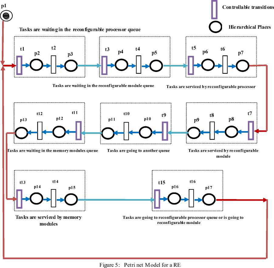
The proposed model for a RE consists of a reconfigurable processor, memory module, and a reconfigurable module. The steps in the reconfiguration elements could be summarized as follows:

• 1.    The tasks are waiting in the reconfigurable processor queue

• 2.    The tasks are waiting in the reconfigurable module queue

• 3.    The tasks are serviced by reconfigurable processor

• 4.    The tasks are serviced by reconfigurable module

• 5.    The tasks are going to the memory queue

• 6.    The tasks are waiting in the memory modules queue

• 7.    The tasks are serviced by memory modules

• 8.    The tasks are going to reconfigurable processor queue or is going to reconfigurable module

This operation is repeated. PN model of reconfigurable processor for a RE is shown in Figure 5.

Corresponding notations are described in table III and table IV.

C.Proposed Model for a Hybrid Processing Element

The proposed model for a hybrid processing element consists of a GPP and a RE. The steps in the reconfiguration elements could be summarized as follows:

• 1.    The tasks are waiting in the CPU queue

• 2.    The tasks are waiting in the reconfigurable processor queue

• 3.    The tasks are waiting in the reconfigurable module queue

• 4.    The tasks are serviced by CPU

• 5.    The tasks are services by reconfigurable processor

• 6.    The tasks are services by reconfigurable module

• 7.    The tasks are going to the memory queue

• 8.    The tasks are waiting in the memory modules queue

• 9.    The tasks are serviced by memory modules

• 10.    The tasks are going to CPU queue or reconfigurable processor queue or reconfigurable module queue.

  
  
  

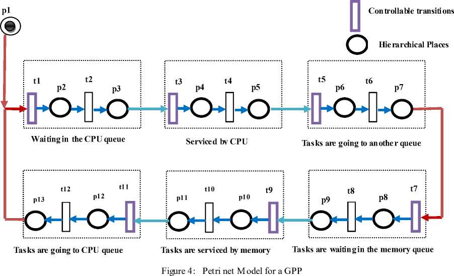
TABLE I. notation for the PN of the Figure 4

Place	Description
p1	Tasks entered in CPU queue
p2	Waiting in the CPU queue
p3	Waiting in the CPU queue completed
p4	Serviced by CPU
p5	Serviced by CPU completed
p6	Tasks are going to another queue
p7	Tasks are going to another queue completed
p8	Tasks are waiting in the memory queue
p9	Tasks are waiting in the memory queue completed
p10	Tasks are serviced by memory
p11	Tasks are serviced by memory completed
p12	Tasks are going to CPU queue
p13	Tasks are going to CPU queue completed

This operation is repeated. PN model of reconfigurable processor for a hybrid processing element is shown in Figure 6. Corresponding notations are described in table V and table VI. Colored Petri nets add another dimension to tokens as well as to selection criteria used in determining firing by the addition of different token types.

Tokens can represent different functions. We can use different tokens to represent operating system calls or different classes of jobs. These different tokens can then be used to determine which transition of multiple transitions available operates.

TABLE II.     notation about transition of the Figure 4

Transition	Description
t1	Start entered tasks in the CPU queue
t2	End waiting in the CPU queue
t3	Start serviced by CPU
t4	End serviced by CPU
t5	Start tasks are going to another queue
t6	End tasks are going to another queue
t7	Start tasks are waiting in the memory queue
t8	End tasks are waiting in the memory queue
t9	Start tasks are serviced by memory
t10	End tasks are serviced by memory
t11	Start tasks are going to CPU queue
t12	End tasks are going to CPU queue

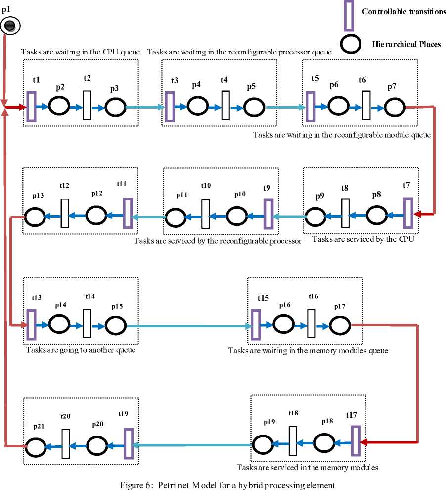
TABLE III.    notation for the PN of the Figure 5

Places	Description
p1	Tasks entered in the reconfigurable processor queue
p2	Tasks are waiting in the reconfigurable processor queue
p3	Tasks are waiting in the reconfigurable processor queue completed
p4	Tasks are waiting in the reconfigurable module queue
p5	Tasks are waiting in the reconfigurable module queue completed
p6	Tasks are served by reconfigurable processor
p7	Tasks are served by reconfigurable processor completed
p8	Tasks are served by reconfigurable module
p9	Tasks are served by reconfigurable module completed
p10	Tasks are going to another queue
p11	Tasks are going to another queue completed
p12	Tasks are waiting in the memory module queue
p13	Tasks are waiting in the memory module queue completed
p14	Tasks are serviced by memory modules
p15	Tasks are serviced by memory modules completed
p16	Tasks are going to reconfigurable processor queue or is going to reconfigurable module
p17	Tasks are going to reconfigurable processor queue or is going to reconfigurable module completed

TABLE IV.    notationabouttransition of the Figure 5

Transition	Description
t1	Start entered tasks in the reconfigurable processor queue
t2	End tasks are waiting in the reconfigurable processor queue
t3	Start tasks are waiting in the reconfigurable module queue
t4	End tasks are waiting in the reconfigurable module queue
t5	Start tasks are serviced by reconfigurable processor
t6	End tasks are serviced by reconfigurable processor
t7	Start tasks are serviced by reconfigurable module
t8	End tasks are serviced by reconfigurable module
t9	Start tasks are going to another queue
t10	End tasks are going to another queue
t11	Start tasks are waiting in the memory modules queue
t12	End tasks are waiting in the memory modules queue
t13	Start tasks are serviced by memory modules
t14	End tasks are serviced by memory modules
t15	Start tasks are going to reconfigurable processor queue or is going to reconfigurable module
t16	End tasks are going to reconfigurable processor queue or is going to reconfigurable module

• TABLE V.     notationabouttransition of the Figure 6

  Places	Description
  p1	Tasks entered in the CPU queue
  p2	Tasks are waiting in CPU queue
  p3	Tasks are waiting in the CPU queue completed
  p4	Tasks are waiting in the reconfigurable processor queue
  p5	Tasks are waiting in the reconfigurable processor queue completed
  p6	Tasks are waiting in the reconfigurable module queue
  p7	Tasks are waiting in the reconfigurable module queue completed
  p8	Tasks are served by CPU
  p9	Tasks are served by CPU completed
  p10	Tasks are served by reconfigurable processor
  p11	Tasks are served by reconfigurable processor completed
  p12	Tasks are served by reconfigurable module
  p13	Tasks are served by reconfigurable module completed
  p14	Tasks are going to another queue
  p15	Tasks are going to another queue completed
  p16	Tasks are waiting in the memory module queue
  p17	Tasks are waiting in the memory module queue completed
  p18	Tasks are serviced by memory modules
  p19	Tasks are serviced by memory modules completed
  p20	Tasks are going to CPU queue or reconfigurable processor queue or is going to reconfigurable module queue
  p21	Tasks are going to CPU queue or reconfigurable processor queue or is going to reconfigurable module queue completed

TABLE VI.    notationabouttransition of the Figure 6

Transition	Description
t1	Start entered tasks in the CPU queue
t2	End tasks are waiting in the CPU queue
t3	Start tasks are waiting in the reconfigurable processor queue
t4	End tasks are waiting in the reconfigurable processor queue
t5	Start tasks are waiting in the reconfigurable module queue
t6	End tasks are waiting in the reconfigurable module queue
t7	Start tasks are serviced by CPU
t8	End tasks are serviced by CPU
t9	Start tasks are serviced by reconfigurable processor
t10	End tasks are serviced by reconfigurable processor
t11	Start tasks are serviced by reconfigurable module
t12	End tasks are serviced by reconfigurable module
t13	Start tasks are going to another queue
t14	End tasks are going to another queue
t15	Start tasks are waiting in the memory modules queue
t16	End tasks are waiting in the memory modules queue
t17	Start tasks are serviced by memory modules
t18	End tasks are serviced by memory modules
t19	Start tasks are going to CPU queue or reconfigurable processor queue or is going to reconfigurable module
t20	End tasks are going to CPU queue or reconfigurable processor queue or is going to reconfigurable module

V. SIMULATION AND EXPERIMENT

The open queuing model in our previous work was validated by computing the average response time results using Maple v.13 analytically and compared with those generated experimentally using OMNeT++ simulator. The service rate of GPP (µ_GPP) varies between 1 and 80, whereas the speedup of RE is taken as 5, Therefore, the service rate of RE was set to 5xµ GPP . Generally, a RE requires a reconfiguration for a set of incoming tasks. In our experiments we assumed that, for each 1000 incoming tasks, one reconfiguration i s needed. The total average error for GPP and RE models for all arrival rates is 2.86% and 2.67%, respectively. These percentage values of error were calculated by dividing total sum of error rates for each model by the respective arrival rates. The simulation results for average response time for all two models are in accordance with the average response time results computed analytically within a range of less than 5% relative error.

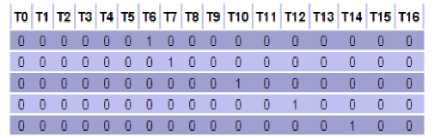
The proposed models were validated by computing the analysis time using PIPEv4.1 simulator. The simulation result shows that Petri net state spaces are bounded and safe and have not deadlock. The average of number tokens in first token is 0.9901 seconds. In these models, there are only 5% errors; also the analysis time in these models is 0.016 seconds. The Petri net invariant analysis results are provided in the table VII.

TABLE VII. petri net invarient analysis results

In our models, there are sixteen places, p0 is first place, and the average number of tokens in each place is depicted in bellow. The simulation results are depicted in the table VIII. The average number of tokens in first place is 0.9901, the average number of tokens in another places is zero. The simulation result in our models is shown that there is 95% confidence interval.

TABLE VIII.   petri net invarient analysis results

Place	Average number of tokens	95% confidence interval (+/-)
P0	0.9901	0
P1	0	0
P2	0	0
P3	0	0
P4	0	0
P5	0	0
P6	0	0
P7	0	0
P8	0	0
P9	0	0
P10	0	0

P11	0	0
P12	0	0
P13	0	0
P14	0	0
P15	0	0

VI. C ONCLUSIONS

In this paper, based on Petri net model, we proposed Petri net models for the processing element. The proposed models can be useful in implementing the real grid networks with RE as one of the processing elements. In our models, the average of number tokens in first token is 0.9901 seconds and there are only 5% errors, also the analysis time in these models is 0.016 seconds.