Analyzing distribution effects of the federal budget transfers for the Far East

One of the main characteristics of modern systems of the federal structure, including the Russian Federation, is the state’s role as a distributor of financial resources between the regions. This role is manifested especially through the system of federal inter-budget transfers. The main recipients of gratuitous grants are usually the regions that have difficulties with replenishing the revenue part of their own budgets. At the same time, all other things being equal, the amounts of the federal aid depend on the severity of the specified problem in a particular subject. On the other hand, the basis for replenishing the fund of federal resources, intended for redistribution, is the part of the regional tax that does not remain at the regions’ disposal. Thus, it does not participate in the formation of revenues of their own budgets.

In economic theory, federal transfers are considered as a part of a fund designed to create expenditure specific to a particular geographical location (region). In this respect, they affect the well-being growth not only of the residents of the territory for which the grants were intended, but also of all other territories, as the latter are also directly involved in the redistribution processes of financial resources of the national economy. Determining the residency, consumers-households can choose the number and types of such benefits provided in certain territories. One of the pioneers of the pure theory of local expenditures, C. Tiebout noted that individuals show their preferences for expenditures through the choice of the “community” – their residency, and there is no way for the consumer to avoid revealing their preferences in the context of spatial economics [1].

Our article is devoted to the analysis of the economic consequences of interregional redistribution of financial resources for the

Russia’ s entities that are a part of the Far Eastern Federal District1, based on a computable general equilibrium model. The latter is a modification of the model used by the author [2] to study the economic effects of resource redistribution in Khabarovsk Krai, and expands its analytical capabilities by adding a block of interregional trade – an aspect that makes significant adjustments to the households’ migration intentions.

The Far East became an object of an active state policy in the 2010s. Designed to ultimately improve the quality of life, business and investment climate, its forms and methods are very diverse. In this regard, it becomes relevant to study the reaction mechanisms of the main economic indicators in the regions of the Far East (welfare, price level, household consumption, etc.) to various aspects of the state economic policy including fiscal policy.

The author was also prompted to continue his work by a recent study of the structure and geographical directions of trade flows in the Far East [3] in which important quantitative results were obtained and systematized.

The model which is the main research tool is an adaptation of the model proposed in [4]. It includes two regions and four economic agents each of which pursues its own economic interests: households, firms, regional governments and federal government. Firms and households demonstrate optimizing behavior: the first maximize profit, the latter – utility (well-being level). The federal government is treated as exogenous, but its actions are subject to budget constraints. Regarding regional governments, there are different assumptions about their target function. It can consist in attracting the population and increasing output, raising the residents’ wellbeing level through expanding the supply of expenditures. The model assumes that regional governments maximize the function of gross public expenditure by setting the tax rate for residents-producers.

Thus, the purpose of experimental simulations is to identify the role of inter-budget transfers in improving the households’ welfare in the Far Eastern regions and the national economy as a whole, as well as their impact on changes in key economic variables: commodity prices, employment, consumption, wages, output, and regional governments’ expenditures.

In accordance with the above, there we set the following tasks: 1) to present the structure characteristic of expenditure and revenue of the consolidated regional budgets of the Far Eastern regions; 2) to give a formal description of computable general equilibrium models with inter-budget transfers which are the basis for simulation calculations; 3) to prepare and justify the values of the original data corresponding to the model constraints.

The model includes interregional trade: part of the goods produced in one entity is consumed by households in another region. However, if in [4] the share of goods, produced in the region, intended for export is set conditionally and the same for all territories, then in our work the corresponding shares are calculated on the basis of [3] for each federal entity of the Far Eastern Federal District. This is the novelty of the research.

The structure of the article is as follows. First, the author gives a description of the budget federalism and its features in relation to the nine entities of the Russian Federation that are a part of the Far Eastern Federal District. Then, the researcher presents an analytical and graphical representation of the two-regional general equilibrium model with factor and trade interregional flows and the federal government. Then there is a model linearization and value assessment of the initial parameters. Finally, a numerical simulation of nine (for each Russia’s entity) variants of the linearized model is carried out by introducing an exogenous shock (federal transfer), and the obtained effects are analyzed in detail.

Budget security of the entities of the Russian Federation constituting the Far Eastern Federal District

Theoretical and economic issues related to the existence of federal grants system include questions related to the optimal size of grants, their impact on the population’s well-being not only in a recipient region, but also in all other regions of the national economy.

In world practice, several models of fiscal federalism can be distinguished [5; 6]. Within the framework of the classical model, territorial entities independently conduct their own fiscal policy in an effort to balance budgets. At the same time, the federal center does not face the task of equalizing the tax potential of the entities, and measures of financial support for the regions are mainly of a program-oriented nature. This model assumes a high degree of management decentralization. A striking example of such a policy is the USA.

The cooperative model of the fiscal federalism is focused on the policy of horizontal and vertical alignment of the budget provision of territories, with a level less than a certain threshold value. At the same time, the regions’ independence in the field of taxation is lower than in the classical model. This model includes the German economy and, to a large extent, the Russian Federation.

The complete elimination of discrepancies between the revenue and expenditure parts of regional budgets seems unrealistic in Russian conditions due to significant differences in the economic and resource potential of the regions, the historically established grid of distribution of productive forces. In Russian practice, the list of performed functions and social obligations of the regional governments is covered only in isolated cases by their financial capabilities [7]. All this requires the higher level of government to provide the missing financial resources to the lower levels (for options for optimizing inter-budgetary relations in the Russian Federation, see [8]).

The role of the federal budget funds in providing the population with state benefits has always been significant for the Far East [9, p. 55]. The share of gratuitous receipts in the structure of revenues of the consolidated budgets of nine entities of the far Eastern Federal District2 ranged from 38% in 2011 to 29.7% in 2018, but it did not fall below 24% during this period. At the same time, the dependence of individual regions on direct federal support varies much more widely. Thus, in the Sakhalin Oblast in 2018, transfers accounted for only 14.5% of its consolidated budget revenues3, while for Kamchatka Krai, depen- dence on the federal funds reached 61%, and for the Chukotka Autonomous Okrug – 62.7%.

Based on table 1 , in the FEFD entities, royalty revenues cover the very different share of total social expenditures in regional consolidated budgets (analysis of balanced budgets, the structure and dynamics of the public debt of constituent entities of FEFD are in [10]). The difference between the penultimate and last columns can be considered as the average per capita volume of expenditures provided by regional governments at the expense of their own income sources. Consequently, given the identity of the average per capita standards of social obligations, the possibilities of regional governments in terms of replenishing the revenue part of territorial budgets are very different.

For the households-residents, the consumption proportions of private and public goods also vary quite significantly from region to region. Thus, in the Primorsky and Khabarovsk krais, the Amur Oblast, the share of gratuitous expenditures in the consumer basket4 ranges from 12.8 to 16.7%, while in the Chukotka Autonomous Okrug this figure reaches 56.7%.

Table 1. Macroeconomic indicators per capita in 2018, thousand rubles

	Salary	Purchase of goods and service payment	Expenses for housing and public utilities and social and cultural events	Gratuitous receipts in the consolidated budget
Republic of Sakha (Yakutia)	362,0	385,1	175,5	83,7
Kamchatka Krai	407,8	398,5	177,4	170,0
Primorski Krai	267,5	331,5	48,5	16,1
Khabarovsk Krai	313,8	395,8	69,4	20,6
Amur Oblast	250,6	299,2	60,1	17,7
Magadan Oblast	544,4	423,2	218,7	96,1
Sakhalin Oblast	458,2	517,6	243,7	46,3
Jewish AO	194,4	228,8	58,3	25,2
Chukotka AO	770,8	353,7	463,0	454,5
Source: Russia’s Regions. Socio-Economic Indicators. 2019 : Stat. Coll . Rosstat, Moscow, 2019. 1204 p.

2 Hereinafter, included in the Federal District at the end of 2018, the Republic of Buryatia and Zabaykalsky Krai are not taken into account.

3 In 2016, even less – 3.5%.

4 The sum of the costs of goods and services and expenditure on housing and utility sector and socio-cultural events.

We also can note a very different ratio between the size of salary and consumer spending. This aspect reflects both the capacity of consumer markets inside each of the Russia’s entities, as well as various opportunities and behaviors regarding savings and spending of monetary income in the current period. We do not analyze the latter aspect in this research5.

It is obvious that even when adjusted for price levels, the differences between the regions in the levels of per capita income are not a determining factor in stimulating labor migration. Such factors include the size of local markets for goods and services noted earlier, as well as the quality of the living environment, play an important role. The latter aspect is indirectly characterized by the level of per capita public spending in the territory which depends on both the size of the tax base and the degree of federal financial support for the regions. The interdependence and mutual influence of all economic agents creates a complex tangle of interactions between them which makes it difficult to assess the impact of external shocks on the behavior of certain economic variables not only in the region itself, but also in the entire national economy. At an acceptable level of abstraction, general equilibrium models allow estimating the direction and (at least) relative scale of such changes.

Setting up a two-regional model with trade flows

The national economic system consists of households, firms, and regional governments, localized in two regions. In addition, there is a single federal government.

There are two types of goods produced – private X and public G. The private ones consist of two goods: the product of region 1 and the product of region 2. Both goods are consumed by households in both regions. The utility function of the representative household in region i has the form :

и = Пл' и; -li; = п№^ (1) 0 < Ун; y2i; 5, < 1, У;, + y2i + 5t = 1, 0 < 0 < 1, where C1 and C2 are household consumption of products from region 1 and 2, respectively, Gi is the amount of available expenditures in region i on average per household, and Li is the number of residents in region i.

In region i , the expenditure provision is ensured in the amount of G_i for all residents-households. At the same time, the volume of public sector services for an individual household is L_i^{1- θ} G_i . The parameter θ is an index of the “individuality” of these services. At θ = 0, expenditures become 100% public when each resident has access to them in full, without reducing the available amount of goods for others. On the contrary, when θ = 1, expenditures are provided purely individually, i.e. they are actually “quasi-public”. In other cases, public goods are “partially competitive”. The article [13] shows that the θG/L value represents the marginal congestion costs, i.e. the price as the form of reduced availability of expenditures to private households, to pay to the resident in connection with the population growth due to migration. It is further assumed that θ = 1.

Each of the Li households in region i offers one unit of labor to the residents-enterprises. As a reward for work, it receives a nominal salary W and a part of the company’s profit in the amount of π. We assume that interregional trade is carried out freely and without costs. This means that the product price from region i is the same for both regions. As the model does not assume savings, all of the household’s disposable income M is spent on purchasing goods. Thus, the budget constraint can be written as:

M i = H i + W i = Р 1 СЦ + P₂C_2b        (2)

Maximization (1) under the budget constraint (2) allows determining the function of individual demand for the benefit of C :

j r.. = YjL Uli     7 = 1?

^C 7 ⁱ 1-S _L P j       ^J 1’2.             (3)

As each household offers firms one unit of labor, L_i is the labor volume supply in region i . There are N companies in the region, and their number is set exogenously. The production process of each of them is characterized by the same production functions with decreasing marginal productivity of labor. We suppose that there is one firm operating in each region, and then the regional issue of Y_i is defined as :

Y_t = L^    0 <  oi_i < 1.           (4)

A representative firm operates under conditions of perfect competition both in the labor and product market. Profit П_i is the value of :

^П - =^PY-WL - ^{(1+ Tl} ),         ⁽⁵⁾

where T_i is the tax rate value charged by the regional government. The model assumes that there is a single tax levied on salaries⁶ and paid only to the respective regional budgets. There are no federal taxes. This assumption makes it possible to simplify the model by excluding the target function and optimizing the behavior of the national government⁷. After substituting (4)

in (5), the profit maximization condition (with respect to L_i ) has the form:

PiCtiLi^"¹ = W i (1 + T i ).             (6)

The part of Y_i output is purchased by the regional government and transformed (with no additional cost) into a local expenditure⁸ GR_i (per household), and the residents of both regions as a private good. We assume that the marginal rate of product transformation between the private and public good is constant and equal to one, as the ratio of their marginal costs is equal to one at any point of the transformation curve ( Fig. 1 ). The governments’ expenditures are covered by their tax revenues. The model assumes that regional budgets are balanced :

piLiGRi = TiWiLi or                     (7)

P_iGR_i = T_iW_i .

The federal government does not formally collect taxes. It redistributes expenditures between regions by withdrawing part of LiGRi (in the amount of LiGFi) from the government of region i and placing it at the disposal of households in region j 9. In fact, intended for gratuitous transfer to the budget of a region, the funds represent that part of the tax revenues of another region that is sent to the federal budget. As far as the model does not assume any other areas of the federal budget expenditures other than interregional transfers, this model technique does not violate the basic principle of redistribution of national income between regions which is the basis of transfers, but greatly simplifies the analysis. The federal government is also balancing its budget:

^Li^GFi = L₂GF₂.              (8)

Thus, the total amount of expenditures provided for the households’ use in region i is:

^Gi= ^GRi ^{+ g r 0      Gi} > ⁰'         ⁽⁹⁾

If region i is the transfer recipient, the expenditure amount available to its residents will exceed the production capacity of the Federation’s entity itself.

Interregional interactions are characterized not only by commodity flows, but also by migration of labor resources¹⁰. Balance is established when the well-being level in two regions is equalized :

01 =

The national labor market has a fixed volume:

12( )

The balance condition in commodity markets implies the distribution of the regional output between local consumption and export :

Y = LiCn + L2C2 + L,GR,.

Condition (12), along with condition (2), implies a zero net of trade balances of both regions. Region i firms distribute all their profits to the region’s residents :

4 = ⁿ , /^L ,                (13)

Finally, the behavior of the regional governments determines the size of T tax rates. ⁱ

In this model, it is assumed that the regional governments maximize their spending under the constraints set by the regions’ production capacity :

n i a x{^L,GR_i} .

The first-order maximization conditions imply:

Li

9GRt

dT ,

9Lt

+ GR,-^ =0, o ⁱt

9GRt        9Lt

- >  0       - <  0 (14)

Q ^T,          QTt

Equations (1)–(14) constitute a two-regional general equilibrium model. The federal government itself chooses the size of one of the GF_i values (for example, GF₂ ), while the second is determined automatically from the budget constraint (8). Thus, the model contains 27 equations and the same number of endogenous variables. In addition to the GF₂ , among the exogenous variables is L .

Before proceeding to the linearized version of the model, the mechanism of the regional system adaptation as a result of an external “shock” (federal transfer) can be shown graphically for clarity. Figure 1 shows a model of the households’ response in region 1 to the receipt of transfer¹² in the amount of GF₁ .

In quadrant 4, there is a residual curve of the region’s product transformation. As the marginal rate of substitution in the production of private and public goods is constant and equal to 1, it is a straight line at an angle of 45°. This curve is called residual because it contains many combinations of public and private goods produced for consumption in region 1 which are achievable after the goods volume, intended for export to region 2, has already been subtracted. If the total volume

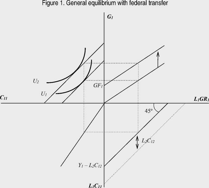
Source: own calculations.

of produced goods remained in region 1 (in the absence of trade), then the maximum volume of produced expenditures (at L₁GR₁ = 0) would be Y₁ . Given the demand of region 2 is fixed at L₂C₁₂ (this value is determined, by virtue of (3), by the households’ income in region 2); the maximum output of the private good of region 1 for its households is Y₁ – L₂C₁₂ .

Quadrant 3 presents the function of transforming the total amount of private good produced for consumption in region 1 into their amount consumed by an individual household. The slope of the straight line here depends on the value 1/ L₁ . Similarly, a function in quadrant 1 is interpreted that transforms the total production volume of expenditure into the value of its individual consumption (a ray coming out of the origin). Its slope is also equal to 1/ L₁ .

Quadrant 2 shows the projection of the map of indifference and budget constraint on the C11 – G1 plane (consumption of local private and public goods). Despite the fact that one of the two goods is free, the budget limit line has a negative slope. Consumption of private goods depends on the amount of household income which, by virtue of (5), decreases as the expenditures production increases. The latter are funded by the regional government, and it is only possible to grow L1GR1 by increasing T1 which causes a reduction in household income.

The federal transfer to region 1 initially causes a parallel upward shift of the function in quadrant 1 by the per capita value of this transfer GF₁ , thereby weakening the household budget constraint. The welfare of the latter grows from U₁ to U₂ . The drift of labor from region 2 causes further transformations in response to the relative change in welfare levels between the regions ( Fig. 2 ).

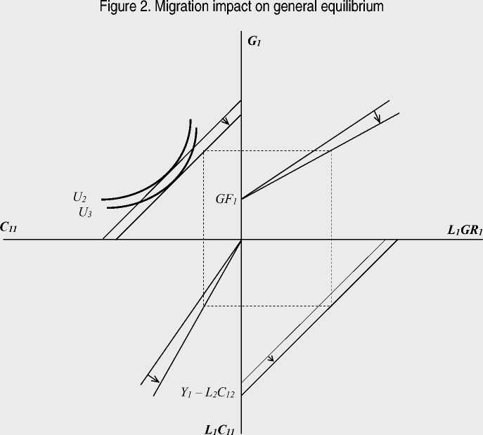
Source: own calculations.

The drift of new labor resources in response to the growth in the well-being level in region 1 will primarily expand the region’s production capacity as a whole. However, the final position of the residual product transformation curve depends on a number of factors. First, the L₂ reduction will reduce the consumption of private good 1 in region 2. Second, the C₁₂ value is affected by income in region 2 and the price level of products in region 1. Their changes caused by the migration process depend on the model parameters. Let us assume that as a result of all the changes, the L₂C₁₂ value has decreased. Then there will be a shift of the residual curve of the product transformation from the origin.

As a result of the increase in labor resources, the slopes of the straight lines in quadrants 1 and 3 will correspondingly decrease (and at the same time their length will grow in proportion to the expanded production opportunities). This will lead to a parallel shift of the budget constraint line to the origin13. The level of household wealth in region 1 will decrease to U3. Thus, the equilibrium system is installed in two stages: first, there is the growth of household wealth in the region through provision of additional expenditures (by reducing household welfare in the second region); secondly, migration to the first region from the second (all other things being equal) reduces the level of well-being in the first.

Linearization and calibration of the model

The model represents a system of nonlinear equations (1)–(14) which makes it difficult to solve it analytically in its original form. It is possible to bring the system to a linear form by logarithmic linearization of equations and then analyze the relative (proportional) changes in model variables as a result of changes in exogenous variables. Equations (1`)–(14`) are a linearized version of the model, where lowercase letters denote proportional changes in variables (log differentials), denoted in equations (1)–(14) in capital letters :

U t = УиСц + Y_2ic_2i + ^ i = 1 , 2 (1)

mt = амп^ + ffMwtWiTihi = —

Ui амт = Щ/Mt, OMwt = Wt/Mt

= "‘i V. = Jt(4')

«iXC (u ₊ ra i/n. (5')

₍          ^/(1+r)

“i;=тг

11 + »Z1 = l, + 8h(8-)

a = ^„,Sr, + telgfl(9')

Oggri = GR i /G i , a_GGFt = G Ri /G t

::=:» : :. 2 )

U1 u2

y t = ^ct i (J i + C il ) : o_YC t2 (l₂ : c t ₂) : : O YGRt ( l i : gr t )

_.= .,.„,

(10`)

(11`)

(12`)

(13`)

Equations (1`)–(14`) form a linear system with 27 endogenous variables c_ij , u_i , m_i , πh_i , п _i , y_i , l_i , p_i , w_i , t_i , gr_i , g_i , gf₁ and two exogenous variables gf₂ and l . The values of the parameters σ follow directly from their definitions and do not need additional explanations.

The next stage of the research is the model transformation into a numerical form by evaluating the parameters and coefficients of the above model. We have built nine numerical versions of the model, according to the number of federal subjects that were a part of the Far Eastern Federal District until the Republic of Buryatia and the Zabaykalsky Krai were admitted to it at the end of 2018. In each of the model variants, the corresponding region of the Far Eastern Federal District acts as region 1, and the rest of the Russian economy (the national economy minus the corresponding subject of the Federation) acts as region 2.

The linearized model version contains a certain number of parameters that should be evaluated. Some of them are contained in the utility function (1`) and the production function (4`). The rest (σ ) are the parameters of linearization. We should pay attention to an important note – the model does not contain a block of savings and investments, as it is inherently static. Meanwhile, real statistical aggregates, on the basis of which parameters should be calculated (consumption volumes, wages and profits, the size of the regional output), also contain “intertemporal” components. Failure to take this part into account will inevitably lead to parameter estimates that are inadequate to the constraints imposed by the model itself. In particular, the total amount of wages and profits (in annual terms) may exceed the annual consumption of households which violates condition (2) of the model. Due to such limitations, the values of a number of economic aggregates used to estimate the model parameters (1`)–(14`), they do not correspond to their counterparts reflected in official statistics.

For the purposes of the research, we add the value of annual regional output Y_i from the sum of regional household consumption L_iC_i and expenditures of regional budgets L_iGR_i on housing and utility sector and socio-cultural activities, minus the amount of gratuitous receipts to regional budgets.

Further, we have made a strong assumption that the profit of π_i (determined from the structure of household income) goes entirely to the current consumption¹⁴. Knowing the values of Y_i , GR_i , L_i (the number of people employed in the economy of the region), and П_i , from the system of equations (5) and (7), it is possible to obtain estimates of the values of W_i¹⁵ and T_i . From conditions (6) and (12), an estimate of the parameter of the regional production function follows :

Y jt =

^C ji

C_u+C_2l+G i '

S t —

G i

C ii +C_2t+G_t'

To estimate the parameters of utility functions (1), it is necessary to consider the values of trade flows between regions that are adequate to the limitations of the model representing a closed national economy. Thus, export and import product flows are not taken into account16. Instead, produced within the national economy, goods and services influence on the household wealth. The total export volume from region i should be equal to the import volume from region j, as we assume that the regional trade is balanced. Instead of arbitrarily setting a fixed share of the value of the private good produced in the region LiCi, intended for intraregional consumption, and applying it to all regions, as some authors have done it [4], we will use statistical data17. As a variable that characterizes the product share of region j imported to region i (dji), the ratio of the volume of product imports to region i from all other regions of the Russian Federation to the value of LiCi is taken. Then:

^L1 ^n — (1 d. 2 ₁)L₁C₁,

L 1 C 21

— d 2 ₁L₁C₁ — L 2 C 12 ,

^L2 C 22

^{— L}2*^2   ^L2 C 12 .

Having estimated the values of C_ij in this way, it is easy to obtain estimates of the parameters of the utility function. Based on the properties (1):

Yjt ^—

^C ji

^C ii ^+C 2i ^{+ G}i'

S t —

G i

^C ii ^{+ C} 2i ^+G i

Finally, the amount of gratuitous receipts to the budget of region i represents the size of the federal grant to region 1 ( L₁GF₁ ). In this case, the condition L₂GF₂ = -L₁GF₁ must be fulfilled to meet the model constraints.

Thus, based on statistical data, we receive estimates of the variables L_i , L_iC_i , L_iGF_i , П_i , L_iC_ji , taken as the arithmetic mean of the values for 2015–2016¹⁸. Then we calculate the values of Y_i , W_i , T_i based on the model limitations. The price indices P₁ and P₂ in the base year take the value 1. The resulting aggregates are summarized in table 2 .

Table 2. Source data for calculating model parameters

	L i C i (bil. rub.)	L i GR i (bil. rub.)	L i GF i (bil. rub.)	LiWi (bil. rub.)	Пi (bil.rub.)	1 – d21	Li (thousand people)
Republic of Sakha (Yakutia) Region 2	153.3 19733.6	83.1 5,129	64.9 -64.9	120.2 17684.0	33.1 2049.6	0.86	483.1 71,762
Kamchatka Krai Region 2	48.4 19838.6	3.8 5208.3	41.6 -41.6	44.6 17759.6	3.8 2079.0	0.60	168.2 72,077
Primorsky Krai Region 2	266.0 19620.9	57.0 5155.1	21.1 -21.1	233.3 17570.9	32.8 2050.1	0.33	975.8 71,269
Khabarovsk Krai Region 2	229.3 19657.6	58.4 5153.7	16.7 -16.7	201.2 17603.0	28.2 2054.6	0.72	688.5 71,557
Amur Oblast Region 2	99.7 19787.2	26.4 5185.7	12.5 -12.5	86.6 17717.6	13.2 2069.6	0.46	394.4 71,851
Magadan Oblast Region 2	33.7 19853.2	14.7 5197.4	9.1 -9.1	30.9 17773.2	2.8 2080.0	0.91	93.6 72,152
Sakhalin Oblast Region 2	117.0 19769.9	94.6 5117.5	5.3 -5.3	99.2 17705.0	17.9 2064.9	0.89	286.1 71,959
Jewish AO Region 2	13.3 19873.6	3.9 5208.2	4.8 -4.8	10.7 17793.5	2.7 2080.1	0.70**	70.0 72,175
Chukotka AO Region 2	8.1 19878.8	2.5 5209.6	14.3 -14.3	7.9 17796.3	0.3 2082.5	0.88	32.5 72,213
* Hereinafter, Region 2 means the national economy except the corresponding entity of the Federation. ** Due to the lack of statistical data, the share of goods and services produced for intraregional consumption is assumed to be 0.7. Source: Russia’s Regions. Socio-Economic Indicators. 2016 : Stat. Coll . Rosstat, Moscow, 2016. 1326 p.; Russia’s Regions. SocioEconomic Indicators. 2017 : Stat. Coll . Rosstat, Moscow, 2017. 1402 p.

Data in table 2 are the basis for estimating the linearization parameters σ , the utility function, and the production function.

Simulation calculations based on numerical model versions and interpretation of the results

In each simulation, one of the nine federal entities becomes region 1, while the rest of the Russian economy becomes region 2. The exogenous effect is an increase in federal transfers to region 1 due to the reallocation of government spending from region 2. Thus, by changing the gf₂ value, the effect of transfers on all endogenous variables of the model can be traced. The magnitude of the exogenous impact should not lead to significant transformations of endogenous variables, as the linearized model version assumes only marginal changes in the values. At the same time, these changes should be sufficient to have measurable results.

In our opinion, such gf2 will be optimal which will provide an increase in ∆GF1 by an amount equal to 20% of the average per capita gratuitous transfers, as at lower values changes in a number of key model variables may be close to zero:

^_GF = 0.2 ^ " ^L i ^GF i _ ¹ L

The average value of per capita gratuitous transfers for 2015–2016 is 22,960 rubles (respectively, ∆ GF_i = 4,592 rubles.). As far as all the entities of the Far Eastern Federal District were grantees during the specified period, the percentage changes of gf₂ have a positive sign in each simulation, but differ in absolute value. We assume that the federal governments direct transfers in order to improve the residents’ welfare of region 1 (from reducing welfare in the rest of the country).

The results of nine simulations, carried out on the basis of a linearized computable general equilibrium model¹⁹, are presented in table 3 .

Table 3. Simulation results

	RS(Ya)	КК	PК	KhК	АО	МО	SО	JАО	ChАО
m1	-0.673	1.624	-1.426	-2.176	-1.420	-0,745	-4.644	-1,082	-0,072
m2	1.500	2.879	1.194	1.576	1.704	2,479	0.946	2,299	0,909
p1	0.964	1.821	-0.553	-0.774	-0.186	0,931	0.706	0,581	0,259
p2	1.495	2.878	1.181	1.563	1.698	2,477	0.938	2.298	0.909
t1	4.162	1.457	3.542	5.264	4.480	5,030	11.798	5.325	1.322
t2	-0.020	-0.004	-0.050	-0.050	-0.024	-0,006	-0.031	-0.005	-0.001
w1	-1.041	1.615	-1.511	-2.321	-1.559	-0,880	-5.524	-1.367	-0.082
w2	1.500	2.879	1.196	1.578	1.705	2,479	0.947	2.299	0.909
y1	1.855	1.160	2.322	3.353	2.783	3,033	5.098	2.853	0.956
y2	-0.013	-0.003	-0.032	-0.033	-0.016	-0,004	-0.020	-0.003	0
y	0.004	0	-0.002	0.006	-0.002	0,002	0.023	-0.001	0
c11	-1.636	-0.197	-0.872	-1.402	-1.234	-1,676	-5.350	-1.662	-0.331
c 21	-2.167	-1.254	-2.607	-3.739	-3.118	-3,222	-5.583	-3.379	-0.981
c 12	0.536	1.058	1.747	2.350	1.890	1,548	0.240	1.718	0.650
c 22	0.005	0.001	0.013	0.013	0.006	0,002	0.008	0.001	0.000
gr1 , l1	2.158	1.252	2.584	3.716	3.107	3,219	5.568	3.377	0.981
gr2 , l2	-0.015	-0.003	-0.035	-0.036	-0.017	-0,004	-0.022	-0.003	0
u1 , u2	-0.007	-0.002	-0.003	-0.004	-0.002	-0,001	-0.003	-0.001	-0.001
нач. u1	0.268	0.267	1.142	0.833	1.025	0,237	0.469	0.720	0.036
gf1	1.244	0.602	18.654	15.216	11.410	1,502	19.252	3.298	0.062
gf2	3.416	1.857	21.273	18.968	14.534	4,726	24.843	6.678	1.043
g1	1.757	0.656	6.918	6.271	5.766	2.564	6.293	3.333	0.197
g2	-0.059	-0.018	-0.123	-0.097	-0.052	-0.012	-0.048	-0.009	-0.003

Note: RS (Ya) – Republic of Sakha (Yakutia), КК – Kamchatka Krai, PK – Primorsky Krai, KhK – Khabarovsk Krai, АО – Amur Oblast, МО – Magadan Oblast, SО – Sakhalin Oblast, JАО – Jewish AO, ChАО – Chukotka АО.

Source: own calculations.

From the point of view of the federal policy, the most important result is a decrease in household utility levels in both regions in all nine variants of the numerical simulation. In other words, increasing federal transfers to these regions is a Pareto-suboptimal solution. However, from a formal point of view, these changes are so small that they can generally be ignored. It should be noted that the effectiveness of redistributive measures is particularly low against the background of significant volumes of GF2 for a number of regions (Primorsky and Khabarovsk krais, Amur and Sakhalin oblasts). Meanwhile, if we consider only the initial change in U1 as a result of the increase in GF1 that followed the transfer from region 2 (line нач. u1 in Table 3), then the effect of redistribution on the welfare of the “indigenous” residents of these regions (before the endogenous change in all other variables including changes in the number of residents) at the initial moment will be positive and quantitatively significant. However, the subsequent changes in other endogenous variables ultimately negate the “gain” of wellbeing.

As for changes in the behavior of regional governments in terms of their fiscal policies, all nine simulations show significant increases in regional taxes T1 and average per capita spending GR1. And to a relatively small extent, this is typical for the Chukotka Autonomous Okrug and Kamchatka Krai. This situation is due to the fact that in these entities the role of the regional governments in providing population with expenditures at the expense of their own sources of income is initially low (see tab. 1). On the other hand, the tax rate and government spending in the donor region were expected to decline in response to the exogenous shock in each of the nine simulations. The Sakhalin Oblast which is characterized by the lowest amount of federal transfers among all the Far Eastern entities of the Federation and the maximum amount of local government expenditures (330.6 thousand rubles per employee), demonstrates a significant increase in the tax rate (11.8%) and the associated increase in local budget expenditures (5.6%).

The result for the Sakhalin Oblast looks paradoxical in light of the fact that the region has the highest basic level of per capita spending GR₁ among regional governments (as a consequence, the highest tax rate T₁ ).

This can be explained as follows. The target function of the regional governments in the model is to increase public spending within their jurisdictions. On the one hand, an increase in the tax rate leads, by virtue of (6), to an increase in labor costs and a reduction in employment, resulting in an outflow of households from the region. This reduces the total costs of the regional government. On the other hand, by increasing tax rate, the government loosens its budget constraint by raising average per capita spending for a given number of households. At the optimum point, the regional government sets a tax rate that balances the impact of the above two effects on total government spending. Receiving the federal transfer will increase the households’ welfare level in the recipient region which will attract additional population to it. To restore the government’s average per capita spending to its previous level, the tax rate will be raised.

The immediate effect of the federal transfer will be the increasing consumption of expenditures in the recipient region, leading to a growth in welfare. The resulting difference in wealth levels between regions will trigger migration processes to region 1 which will stop when these levels become equal again. Thus, the growth in the labor force in the recipient region and its reduction in the donor region will be a clear result of the redistribution of financial resources.

The dynamics of the number of labor resources is directly related to the output dynamics. Due to the properties of the production function, the increase in total output in region 1 will be less than the employment gain, while for region 2, the decrease in output is lower than the employment decline (at least in those simulations where the effect is statistically noticeable). As for the output per employee ( y_i – l_i ), the donor regions will be characterized by its reduction as a result of the federal transfer. It is also interesting to follow the changes in the gross output of country y . As table 3 shows, migration has a dual effect on this indicator – in four cases it is positive, in three – negative. In two other cases, the impact on the value of national output is not observed.

Federal transfers also have an impact on price changes. In three recipient regions (Primorsky and Khabarovsk krais, the Amur Oblast) the price level of local production p₁ has decreased. Characteristically, in all simulations, there is an increase in prices for the products of the donor region, and more significant than for the recipient region (for cases where p₁ , p₂ > 0). Changes in prices are also associated with transformations in interregional trade. It is worth noting rather significant reduction in the average per capita consumption of products of region 2 by the recipient region. On the contrary, residents of the donor region take the average per capita consumption of goods in region 1.

The value c₂₁ + l ₁ characterizes the change in the import of region 1 from region 2. Accordingly, c₁₂ + l₂ reflects the export dynamics from region 1 to region 2. It follows that, in general, the import volume of goods to the recipient regions practically does not change (formally speaking, c₁₂ + l₂ is reduced within thousandths of a percent). On the contrary, the products export from the recipient regions to the donor region raises significantly (in some cases – more than 1.5%). As far as interregional trade is balanced in the original model, the difference between these values gives a percentage change in the trade balance. Thus, in all tested cases, federal transfers improved the terms of trade in favor of the recipient regions.

The above effects can justify in the following way. The reduction in output per employee in the recipient region results in a reduction in salaries, profits and, as a consequence, the income of a representative household in region 1. This will lead to a reduction in the specific consumption of both goods. Similar, but with the opposite sign, processes cause an increase in per capita consumption in region 2.Thus, there will be a reduction in demand for product 1 in region 1, but an increase in demand for it in region 2. However, in a number of cases (Primorsky and Khabarovsk krais, the Amur Oblast), the total excess supply of local goods in the national economy will lead to a drop in prices for them.

The model calculations, the results of which are shown in table 3, are carried out under the assumption that regional governments set the tax rate in such a way as to maximize their spending in the region. The question arises whether the results of calculations strongly depend on this premise. A comparison can be made with the results of simulation under the assumption that the behavior of regional governments is set exogenous. In this case, equation (14`) is replaced by the condition gri=0. Therefore, Ti is determined based on maintaining the budget constraint of regional governments.

Based on the evaluation results within the framework of this option, it is impossible to say unambiguously that there is a trend in changes in indicators. In the case of the Republic of Sakha (Yakutia), Magadan and Sakhalin Oblasts, the new results were unrealistic (the values of changes in individual variables for both region 1 and region 2 were 20% or more). For the Kamchatka and Primorsky krais, the Amur Oblast, the signs for all variables remained the same as in table 3, but slightly decreased in absolute value. Finally, for the Khabarovsk Krai, the Jewish AO, and the Chukotka AO, the signs for the variables for the recipient region did not change, and for the donor region, most of the variables changed the sign to the opposite. For the last two groups of regions, there is a weak tendency to increase welfare if regional governments behave as agents that maximize their budget spending functions.

Conclusion

The article analyzes the effects of interregional transfers for the regions of the Far East carried out by the federal government, using a two-regional computable general equilibrium model with optimizing regional governments. Nine numerical simulations were carried out on the linearized version of the model the parameters of which were calibrated using statistical data for nine federal entities of the Far Eastern Federal District for 2015–2016.

We have found that federal transfers have almost no effect on household welfare, but lead to significant changes in other economic variables. Despite the essential initial increase in the residents’ welfare of the Far Eastern regions as a result of the growth in the value of federal transfers, the households’ ability to optimize their consumer basket and migrate from region to region in response to the difference in utility levels ultimately leads to the leveling of the resulting benefits. It is achieved at the cost of significant changes in the levels of prices, wages, output, tax burden, and regional budget expenditures, primarily in the recipient regions. The initial increase in wealth leads to an influx of labor resources, lifting output, but reducing labor productivity and salaries. Regional governments respond to the population’s influx by increasing the level of budget expenditures through tax rate growth which puts additional pressure on salaries and incomes of residents, reducing their consumption level. In the end, welfare returns to its original level and a new equilibrium is established at a lower level of prices and average per capita income in the recipient region.

From the point of view of the federal government, the most pronounced effect will be the migration toward the regions receiving federal grants, as a result – the GRP growth of the latter. It should be clarified, however, that all estimates are based on the assumption that the price level in both regions is equal in the initial period ( P₁ = P₂ = 1) which is not the case in reality²⁰. It follows that the decline in cost indicators in the recipient regions should be interpreted only as a slowdown in their growth rates compared to the national average.

As we have already noted, the model is static in nature and considers households as agents aimed at current consumption. Consequently, their motives for future consumption and savings are not taken into account. However, it is widely believed that the main motive for migration to the Far East is the ability to expand the budget restriction of future periods in order to increase future consumption. This is true if we assume that consumption consists only of private goods, whereas, according to the same neoclassical theory, the comfort level and convenience of living provided by the presence of expenditures is an incentive to change the location [16].

An important conclusion that confirms the earlier ones [3] is that the Russian Far East does not represent a homogeneous integral economic system that could be described as the “economy of the Far East”. In fact, the Far Eastern Federal District is a set of federal entities characterized by different natural and geographical, demographic, structural and economic conditions that do not determine the overall single common market. In addition, the research allowed supplementing this description of the macroregion with the following feature: the constituent entities of the Far Eastern Federal District are characterized by different reactions and different, sometimes having the opposite direction, effects in relation to the policy measures of resource redistribution.