Analyzing progressive-BKZ lattice reduction algorithm

Lattice of our interest is integer or point lattice; discrete subgroup ofR ” . It is defined as the integer linear combinations of some vectors (b i , . Ь д ) of the form: ^ f=₁ x _i .b _i where x , EZ are the integers. The vectors (6,..., Ь д ) are linearly independent and called a basis of the lattice. The number of vectors d is the lattice dimension.

The goal of lattice reduction is to find good and quality bases that include short enough vectors. SVP or Shortest Vector Problem is the most common and fundamental lattice problem on which many cryptosystems rely on. In lattice-based cryptanalysis one typically looks for an approximate variant of SVP, i.e. to obtain a vector ~ a X Л 1 (L), where d is the dimension of lattice L , a > 1 is the approximation factor and Л 1 (L) is the first minimum (the length of the shortest nonzero vector of L). Another important lattice problems are CVP (Closest Vector Problem) and SIVP (Shortest Independent Vector Problem).

Lattice problems are considered as a key element in many areas of computer science as well as cryptography. In particular, public key cryptosystems based on knapsack problem, special setting of RSA and DSA signatures schemes; encryption schemes based on LWE (Learning with error) problems; fully homomorphic cryptosystems are the most important.

Hash function SWIFFT [1], consists of following compression function:

T^Oi.XtER where R = ^ ^ is the ring of polynomial, ai E R (for all

• i)    ar m fixed multipliers and  X i ER (Vi) with

coefficients E {0,1} are the input of length mn. Other parameters of this function include n be a power of 2 and a prime modulus p > 0. The algebraic formulation of SWIFFT is equivalent to a lattice of dimension mn and the security of such function depends on the infeasibility of finding relatively short vectors in such a lattice. Finding a collision in this function means to look for a nonzero vector X i E R with coefficients are in {-1, 0,1} such that X /=i d i - X i = 0 mod p. In other words, if we can find a vector by reducing the lattice (considering a sublattice of dimension m ' n ' < mn will be enough) of Euclidean length < Vmn, then it is called pseudocollision .

The most efficient (in terms of reduction quality) BKZ lattice reduction algorithm can able to find such collision in 2o(d2) time complexity. Both theoretically and experimentally we show the variant BKZ-Progressive can do so in reduce amount of time. Precisely, in section IV we give a heuristic argument that it has enumeration time complexity of nearly 20(d Zos d)+0(d). In section V we plot experimental results to support this proposition and in section VI we provide its average runtime complexity for finding pseudo-collision in SWIFFT comparing with BKZ. We also showed that it can achieve the quality of reduction as good as BKZ.

• II.    Related Works

  Lattice reduction technique has been studied from the language of quadratic forms (by Hermite in 1850 and then by Korkine-Zolotarev in 1873, together combine HKZ reduction) to analyze current cryptosystems. But it

  is not seemed to have much improvement since Lenstra-Lenstra-Lovász seminal LLL [2] algorithm has been published in 1982. This polynomial time algorithm is very fast with moderate reduction quality to solve shortest vector problem (SVP). In [3], Schnorr introduced the block concept of HKZ reduction to produce the best reduction algorithm (BKZ) in practice until today. This algorithm gets much slower when block size increases but can achieve approximation ratio (Hermite factor) upto ~ 1.011 ” while LLL can achieve roughly upto ~ 1.022 ” according to [4]. The practical BKZ algorithm is reported in [5] and has been since widely studied by researchers related to this field. Both LLL and BKZ is implemented in NTL package [6] and usually used as a base of any relevant experiments.

Quasi-HKZ reduction technique proposed by Ravi Kannan [7] is another celebrated work that achieve best theoretical bound on enumeration procedure (lattice reduction technique often combines with enumeration routine, for example in BKZ reduction algorithm). An improved analysis of this algorithm is reported in [8] by Stehle´and Hanrot. Recent significant improvement is done by Gama et al. in [9] where they introduce extreme pruning concept for enumeration. This leads lower success probability to find a short enough vector but gain in overall by saving considerable time. Gama and Nguyen’s experiments done in [4] suggest some actual behavior (output quality vs. running time) of lattice reduction algorithms to reduce the gap between theoretical analysis and practical performance of lattice algorithms.

We believe there are two variants of applying BKZ progressively. The first variant uses same lattice basis with increasing block sizes to look for a particular lattice reduction quality. In [10] Buchmann and Lindner used this approach to find sub-lattice collision in SWIFFT, similar approach is used in [11] by Lindner and Peikert to extrapolate BKZ runtime for LWE parameters. The other variant (feed forward approach, i.e. the output of current block is used as the input of next larger block) that used as a preprocessor of the enumeration routine in [12] designated as recursive-BKZ. Our definition of Progressive BKZ is believed to be substantiated the later variant.

• III.    Preliminaries

• A.    Gram-Schmidt Orthogonalization

The purpose of lattice reduction is to search for orthonormal basis i.e. look for the unit vectors that are pairwise orthogonal in the basis. Gram-Schmidt orthogonalization method can always transfer a basis В = (b _i , ..., b _d)into orthogonal basis В = (b i , ..., Ь Д ) as follows:

bi = bt b* = bt ^ [iub]

t>]

where Дц = (b_t, b y )/^ * , b ] ) for all i ^ j. We can also define the orthogonal Gram-Schmidt vectors as b - ~ n t (b i ) for all non-negative i < d, where t _t denotes the orthogonal projection over the orthogonal supplement of the linear span of b_i, ..., b - (see [13] for details). Every lattice reduction algorithm uses this process to find the reasonably short lattice vectors.

• B.    Input and Output basis

The basis that is chosen for SWIFFT can be represented as the following matrix:

hhл)

where H is a n X n * (m — 1) skew circulant matrix in Zp = 0.p — 1 and p is the prime for the SWIFFT parameters. 7 is the n * (m — 1) X n * (m — 1) identity matrix. Right bottom is the n X n scalar matrix and right top is a n * (m — 1) X n dimensional zero matrix.

According to [9], sufficiently random reduced bases except special structure have a typical shape for main algorithms like LLL and BKZ and the shape depends on the ratio q = ||b * ₊₁H/Hb_t * Hof Gram-Schmidt vectors. This follows Schnorr’s Geometric Series Assumption (GSA) [14]. The running time of the algorithms depends on q. The BKZ-Progressive also produces same shape as BKZ for certain parameter choice (m ' < m) of the input basis. As m' increases (fixing the n') the ||b_t * H ' s produce a constant 1 consistently, i.e. the ratio q is 1 too. Seemingly, we can say as long as the basis does not produce special structure the shape is typical. From the discussion of [11] we predict the q reaches its lower bound 1. Now on we will mention the first case as the typical behavior of ||Ь * П as well as q and the second case as special behavior. We discuss both cases while analyzing BKZ-Progressive performance and SWIFFT in later sections.

• C.    Enumeration

Enumeration is a technique that is used alongside lattice reduction for most of the major algorithms. If we imagine a lattice L as a tree, then enumeration procedure is simply an exhaustive (depth-first) search for integer combination of the nodes (or vectors) within a upper bound in A1 (L). This procedure (also implemented in NTL) run in exponential time opposed to the lattice reduction technique itself (which run in polynomial time).

• IV.    Theoretical Motivation for BKZ-Progressive

Block-Korkine-Zolotarev reduction a.k.a BKZ reduction is the most successful lattice reduction algorithm in practice. Schnorr and Euchner [5] introduced the following dentition of BKZ reduction.

• A.    BKZ Reduction

Let в be an integer such that 2 < ^ < d. A lattice (L) with basis (Ь₁,.,Ь д ) is в -reduced if it is size reduced and if (for i = 1,..., d — 1)

Hb*H <Л1 (n,(L(bi b^^-^))))

Ravi Kannan provides an algorithm that computes HKZ reduced bases to solve SVP. The main idea of Kannan’s algorithm is to spend more time on precomputing a basis of excellent quality before calling the enumeration procedure. Our BKZ-Progressive approach inspired from Kannan for pre-processing a basis of subsequently increasing block size can be defined as follows.

BKZ-Progressive Reduction : Let BKZ (d,/?) denotes the BKZ algorithm running on a lattice dimension d with block size в. Instead of reducing BKZ (d,/) in the first place it will reduce the basis with smaller block size upto в with BKZ(d, 2), BKZ(d, 4),..., BKZ(d,/).

• B.    Heuristic

A d- dimensional lattice reducing with BKZ-Progressive approach requires enumeration complexity of approximately 2^{0(k 100 k)} , where k is the block size.

Proof. For BKZ reduction with block size k the recent theoretical analysis (see Theorem 2 in [15]) shows that

,        log (y)

logq к 1

where y <  c _h * к is the Hermite constant in dimension k (for constant c ^ ). The number of BKZ- k iterations enough to get this log q is <  ( c' * И³/к² ) for constant c ' . Since progressive BKZ applies (for t = 2,4,..., к — 2 ) BKZ—(t + 2) on an input basis which is the output of BKZ-(t) , we expect the enumeration time for BKZ—( t + 2) to be (from the heuristic estimation described in [13] for solving SVP using enumeration)

q C⁽i+2^{) 2} = 2 log⁽c _h .i⁾/⁽i-1⁾.c.⁽i+2^{) 2} = 2 C.Zo0(ch.i)(i+O(1))

where c is another constant. Since < c’ * n3/ (i + 2)2 iterations needed for BKZ—(t + 2) for t = 2,4,..., к — 2, the total enumeration time (T) for BKZ-Progressive would be

T < y._r' ⁿ 2   СсОод^снДроодУ)

¹ < ^LiL (i+2) 2 2

< ^c' И 2 C ^O0(c h ,^)(^+O(1)) < 2 O(k.^O0fc)

• V.    Experimental Result

Experiments are done in 2.67 GHz Corei5 (64 bit) Intel processor machine. The BKZ algorithm and associate enumeration routine is the NTL implementations of floating-point version.

• A.    Reduction Quality and Shape of Hb * Н

The reduction quality of lattice basis depends on the Gram-Schmidt vector ||6 * H, for a good reduction algorithm the value of ||6*|| does not decay too fast. The parameter q = Hb * _o1H/Hb_i * H is the measure of a lattice reduction quality. According to [13], for LLL reduced basis q = 1.04 (in high dimension) and for BKZ-20 reduction the value is equivalent to 1.025. The slope of the fitted logarithmic linear curve of ||6 * H is also a measure of reduction quality.

s data for BKZ-Progressive fitted curve: c^t log(k) /(k-1) — c =0.0265, c =0.02231

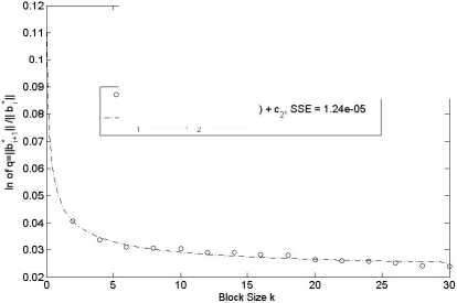
Fig.1. Reduction Quality in BKZ-Progressive on an Average.

Table 1. Root -Hermite factor that can be achieved in BKZ-Progressive Reduction with Dimension 120.

k	q	δ
2	1.04154	1.02038
4	1.03415	1.01678
20	1.02672	1.01316
22	1.02637	1.01298
24	1.02608	1.01284
26	1.02538	1.01250
28	1.02453	1.01208
30	1.02423	1.01194
32	1.02390	1.01177

In BKZ reduction approach the block size is the parameter that controls the reduction quality. Larger block size gives better reduction in increase of runtime. That means the ratio q should get lower when the block size increases. Experiments done by Gama and Nguyen in [9] (using CJLOSS lattice) found slope = -0.085 for LLL reduction and -0.055 for BKZ-20 reduction (in dimension 110) consideringHb * H 2 instead of Hb * H. Figure 1 shows in our case, how the log q (the slope) decreases in increase of block size. A fitted curve for the data points also satisfy that log q — log к/(к — 1) (which supports our theoretical assumption for enumeration time).

The better reduction directs us to the closer approximation to the shortest vector. The best current Hermite factor (5^й = Hb₁H/VvOT)L) is reported in [4] is about 1.0109^d for BKZ-28 reduction. As we know

(d+1)

q 2  = 5й for lattice dimension d, the relation between q = ||b*o1H/Hb*H and root-Hermite factor is approximately 5~^^. Table 1 shows our experimental outcomes for BKZ-Progressive reduction. The tabulated values are of q, and root-Hermite factor for different increasing block sizes (k) of dimension 120.

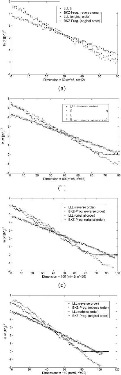
It is to be said that the slope of the fitted HbfHcurve will be independent of lattice dimension. But it is true if the Gram-Schmidt norms HbfH behaves typically. For our SWIFFT input basis setting we performs experiments to see how the order)

(b)

(d)

Fig.2. Shape of Hb f H curve Changes as Dimension (in (a) = 60, (b) = 80, (c) = 100 and (d) =110) Increases.

ILL (reverse order,» BKZ-Prog. (reverse order LLL (original order) BKZ-Prog, (original order!

actual shape of Hb f H looks like after different reduction approach in increase of dimension. We want to see in what dimension the transition (typical to special case) occur and whether the shape of Hb f H changes differently when we consider change in input basis vector’s order. Figure 2 plots this idea. Let us say i ' is the dimension after which a transition from typical to special case occurs i.e. Hb f H (for i >  I’) becomes constant 1. Also, the current input setting (as in section III) is considered as original order of basis vectors and a reverse setting of these vectors is considered as reverse order. For original order i ' denotes as i '_old and for reverse order i ._ew .

For BKZ-Progressive output, the curves of log Hb f H are about the same for both orders and are straight line of gradient log (q) for i < logHb f H = 0 for both orders. For LLL output, in the reverse order, log Hb f H is approximately a straight line with gradient log (q) for i <  i ._ew , where i ._ew is the value of line for which the straight line intersects zero. For i > i . _ew, log Hb f H =0 in this order. In case of original order, log Hb f H is a straight line of gradient log (q) for i in the interval i . _ew > i < if^ (with same values of log (q) and i' as in reverse order). For i > i ’_M , logHb f II = 0 for i < i .ew ,logHb f П is roughly a convex curve above the straight line of reverse order, intersecting this straight line at i = 1 and i = i . _ew + 1 (i.e. logHb f H)is approximately same for original and reverse orders and logHb f H=0 for both orders). Also, i' is about the same for BKZ and LLL output (see (c) and (d) of Figure 2).

• B.    Enumeration Time Analysis

We know BKZ reduction procedure implemented in NTL consists of two main parts; enumeration segment which performs exhaustive search in enumeration tree and the reduction segment calculates the enumeration time per iteration or block. For progressive approach of BKZ —k reduction, while BKZ-2, BKZ-4,...,BKZ-k reduction is performed subsequently, we consider the last block’s enumeration time (i.e. BKZ-k) to compare with that of BKZ only approach. Figure 3 gives a comparison graphs for these two approaches. We consider here dimension 120 with a Schnarr-Horner pruning [16] parameter 1 to allow larger block sizes.

Least square fitting for the data points of these approaches generate different curve fitting models. In case of BKZ, the fitted model is /(k) = 0.017 * k2 — 1.1 f k + 16 with SSE (Sum of Squares due to Error) equivalent to 0.98. On the other hand, BKZ-Progressive fits model/(k) = 0.44 f k f ln(k) — 1.8 f k + 5.9 with SSE = 0.25. An alternative model /(k) = 0.062 f k f ln(k) — 11.25 also fits quite well with SSE only 0.64.

The above models are generated for special case of Hb f H, for a typical case scenario we get a similar model for BKZ-Progressive approach (/(k) = 0.61 f k f ln(k) — 2.6 f k +14 with SSE = 0.006).

It shows an improvement over the Peikert-Lindner work in [11] where they used BKZ with block size k directly on LLL reduced basis (default NTL-BKZ implementation), hence resulting in expected BKZ block enumeration time exponential in k2. We pre-process the basis before applying BKZ-k by progressive BKZ procedure, resulting in a lower time on the exhaustive search condition. During such a search for the short vector, the enumeration segment is executed number of times. This is the total number of iterations for a BKZ-k reduction. Knowing the total time for those iterations for a block size k, we can expect BKZ block enumeration time is exponential in k * log( k).

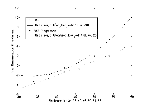
Fig.3. Average Enumeration Time for BKZ and BKZ-Progressive

• VI.    Cryptanalysis of SWIFFT

  Again, to obtain pseudo-collision we need to find a vector of norm 06 1 0 (usually the first vector in the reduced basis) in such that 06 1 0 <  ^mn. Following [13] we can calculate the value of 06 1 0 for certain parameters (d, n, p and q as their usual meaning) as follows:

06 1 0 ~ q^(d-1)/2vol(L)^1/d ~ q^(d-1)/2£yp "     (1)

Where vol(L) is the volume of lattice equivalent to the determinant of it (= pⁿ). The usual parameters choice for SWIFFT are m = 16, n = 64 and p = 257 .

• A.    Models for Typical and Special Case

  In typical case the graph of log of 06 1 0 versus i (for i = 1,..., d ) is a straight line with gradient log (q) (that depends on the block size k). This means that

logHb * H = logH^ i H — ⁽i - 1) * logq       (2)

Since we know that

Z d=i ^ogHb r H=log(vol(L))         (3)

Substituting (1) in (2) gives us logHbiH = (d — 1)/2 *log+1/d *log(vol(L)) (4)

This is the relation we have in equation (1). From (4) and (2), we can see that the quantity 1/d * log(vol(L)) is approximately equal to 06*0 for i ~ (d — 1)/2, i.e. the straight     line     crosses     the     value 1/d *

log(vol(L)) approximately in the middle. This means the lowest value of the line, log 06 1 0 is about 1/d* log(vol(L)) — (d + 1)/2 * log q . So, the condition for the typical case should be that log06 d 0 > 0- Then for the special case, log 06 * 0 falls with a gradient log (q) for i = 1,..., i ' (where i ' < d) and log 06 * 0 = 0 for i > i'. Then using (3) we get the following relation in place of (4):

log06 i 0 = (i' — 1)/2 * log q + 1/i' * log(vol(L))   (5)

Similarly, to the above, (5) means that log06*0 = 0 = 1/i' * log(vol(L) — (i’ — 1)/2 * log which is quadratic equation in i' as a function of log q and vol(L). By solving this equation, we get a model for i'. These have been used to find the pseudo-collision in following section.

• B.    Pseudo-Collision Parameters

  Micciancio and Regev in [17] first observed experimentally that shortest vector of length l = 2² V ^nlog P ^log5 can be obtained for an optimal dimension d = ^nlogp/log 5. Based on this idea, in our case we can only satisfy the condition of pseudo-collision for much smaller n ' (n = 20)- The other parameters we consider are 5 =1-0117 and p = 257 fixed in our case. For larger n, a successful collision is not possible if we restrict these parameters. A smaller choice of parameter p and 5 can obviously find collision for larger n (as well as d). In fact, in [10] a smaller choice of modulus p has been considered for pseudo-collision estimate.

Table 2. Choice of Parameters for finding pseudo-collision in Special Case.

d	m’	n'	p	k	q	06 1 0	06 1 0 ’
96	6	16	257	4	1.03415	11.54	9.70
108	6	18	257	10	1.03081	11.60	10.10
120	6	20	257	12	1.02946	12.52	10.58
140	7	20	257	14	1.02934	12.53	11.57
151	7	22	257	18	1.02811	13.55	12.28
168	7	24	257	22	1.02637	13.89	12.85
175	7	25	257	21	1.02608	11.19	13.22
182	7	26	257	28	1.02538	15.60	12.20

We certainly cannot decrease the value of 5 as it is reported from [4] as optimum for current best algorithms and our experiments (in Table 1) support this. However, it would be somewhat different if we considered the special case shape of 06*0 and extract gradient log q from this shape instead of straight-line model. But a close investigation reveals that a situation like special case happens when the input vectors are smaller in length (i.e. for larger m and smaller n') in the basis. Experimental estimate of pseudo-collision is listed in Table 2 where eight different instances can launch successful attack in feasible time. We plot experimentally derived norm of shortest vector value in column ||61||’, H^1H entries are for theoretically derived shortest vector value. It is calculated by the i' < d from experimental data and then plugging into the model for special case. We see that the experimental result is better than the theoretical one. We can reach up to n = 27 within the time around 9.5 hours. We record the runtime to obtain pseudo-collision in both BKZ and BKZ-Progressive approach. Figure 4 shows the comparison graph.

• C.    Pseudo-Collision in Typical case o/ ||6_t*||

However, it might be interesting to see what experiment can achieve in perfect typical case condition. We found the following entries (in Table 3) that satisfy the pseudo-collision constraint. To derive the value of q for corresponding larger value of к we used linear extrapolation.

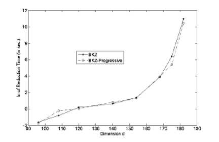
Fig.4. Average Runtime for pse udo- collision .

In this case, it is hard to get a pseudo-collision as we cannot able to increase the value of m' <  m much (as its give shape like special case) and if we increase n we rarely find a short vector as volume of lattice jumps high. Again, in this situation we need to decrease modulus p to become successful.

Table 3. Choice of Parameters for finding pseudo-collision in Typical Case.

d	m’	n'	p	k	q
90	5	18	257	26	1.02538
100	1	25	79	28	1.02153
114	3	38	29	44	1.02210
120	3	40	29	50	1.02120

The runtime for first two instances ( d = 90 and 100) of BKZ reduction requires approximately 185 and 1170 seconds on average. On the other hand, BKZ-Progressive can reduce the instances for 92 and 575 seconds respectively on an average. So, the time improvement is about a factor of two. For other instances, as the block size and dimension both become increasingly high it is unexpected to get collision in feasible time.

• VII.    Conclusion

In this paper, we investigate the performance of the Progressive approach of BKZ lattice reduction in which an enumeration-block is preprocessed by the immediate previous block expect to improve the reduction time. We analyze and compare its performance using real lattice basis. Finally, we show an attack ( pseudo- collision) on SWIFFT hash function that is based on Lattice problem.