Anomalies in IGS ephemeris and clock products and their influence on the solution of navigation problems

The problem of precise point positioning (PPP) is of great importance in geodesy and is one of the ways to use global navigation satellite systems (GNSSs). To solve this problem, phase and code measurements from a navigation receiver as well as updated information about the orbits and clocks of navigation satellites are used. The analytical centers of the International GNSS Service (IGS) [1]: IAC GLONASS [2], CODE [3], ESA [4] and others are a source of information about the updated (final) orbits and clocks (frequencytime corrections to the satellite time scale). Information about the orbits is transmitted in the SP3 format for each daily time interval in the form of time series of data with a time step of 15 min [5], information about the satellite clock is transmitted in the CLK format with a time step of 30 s or 5 min [6]. The method for detecting anomalies in orbits used by us was previously described in detail in [7; 8] and allows detecting small (centimeter) anomalies in the orbits of navigation satellites. Also, in [7] it is noted that at the boundaries of daily intervals there are often discontinuities ("jumps") in orbits. It is not difficult to detect anomalies in clock drifts: it is enough to remove linear and quadratic (for large time intervals) trends using the least squares method (OLS).

We made attempts to "correct" the detected orbit anomalies, that is, to correct the orbit so that a new orbit would not have a discontinuity at the boundary of the day and would be close to the published final orbits. However, such a correction did not always lead to an increase in the positioning precision or worsened it. This is due to the presence of similar anomalies in the time information (the NS clock drift).

Orbit anomaly detection method

The technique for anomalies searching in SP3 data (standard text format for ephemeris IGS products, available in daily intervals with a step of 15 min in time) consists in searching for orbital discontinuities (time series jumps) at the boundary of two daily intervals by approximating each of the satellite coordinates for this two-day interval by a high degree polynomial. Next, the approximation residual is calculated. As it is shown in [7; 8], from the obtained residual it is easy to determine the type of anomaly ("jump" or "ejection", as well as the satellite maneuver or the period of entering the shadow). The approximation method we used is based on the application of a precomputable set of discrete orthogonal Chebyshev – Khan polynomials [8]. Such polynomials are calculated in timestamps of the analyzed series up to the chosen degree r (in our case, r = 100), after which the polynomial of the best RMS approximation is easily calculated. The main problem is calculating Chebyshev-Khan polynomials. The standard formulas of the theory of orthogonal discrete polynomials are not suitable due to the accumulation of large errors for high degrees and with a large number of points (in our case, 192 points). Stable algorithms for computing Chebyshev – Khan polynomials are described in [8]. In this work, we used a software package [9] adapted to the problem of approximating orbits. The method of polynomial approximation is much simpler than the approach considered earlier in [10; 11], which provided for high-precision modeling of the motion of the NS by solving the equations of motion using a lot of additional data.

For the precise positioning problems we are solving, not the orbital anomaly along each individual coordinate is important, but the value of its projection onto the sighting axis between the satellite and the receiver. To simplify the analysis, the center of mass of the Earth was used as the coordinates of the receiver, i.e., the value of the anomaly was calculated along the radius vector of the NS - the center of the Earth.

Anomalies detected in IGS final orbits

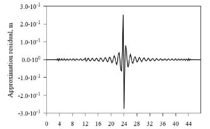
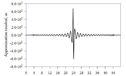
The issue of anomalies in the orbits of navigation satellites is discussed in [7; 8; 10; 11]. The work [7] shows the detected anomalies in the orbits of GLONASS satellites; the same anomalies are observed in the orbits of GPS satellites. The examples of the detected "jumps" in the final orbits of satellites G03 and G08 at the boundary of the day (more precisely, their effect on the approximation residuals) according to the IAC PNT analytical center are shown in Fig. 1 and 2.

Tune from the beginning of the two-day interval. h

Fig. 1. Approximation residual of the G03 satellite Y coordinate by the 1 00 ^th degree polynomial at the day boundary 21–22 November 2014 by the IAC PNT

Time from the beginning of the two-day interval, h

Fig. 2. Approximation residual of the G O8 satellite

Y coordinate by the 1 00 ^th degree polynomial at the day boundary 5–6 April 2018 by the IAC PNT

Рис. 1. Невязка аппроксимации полиномом степени 100 координаты Y спутника G03 на стыке суток 21–22 ноября 2014 г. ИАЦ КВНО

Рис. 2. Невязка аппроксимации полиномом степени 100 координаты Y спутника G08 на стыке суток 5–6 апреля 2018 г. ИАЦ КВНО

According to the recommendations given in [7], we determine the size of the "jump" at each boundary of the day. For the approximation residual shown in Fig. 1, the magnitude of the "jump" is about 70 cm, for the approximation residual in Fig. 2 the magnitude of the "jump" is about 1.8 km. Large "jumps" in the final orbits of analytical centers are not very common (on average 1 "jump" per year for each satellite), while small "jumps" are common.

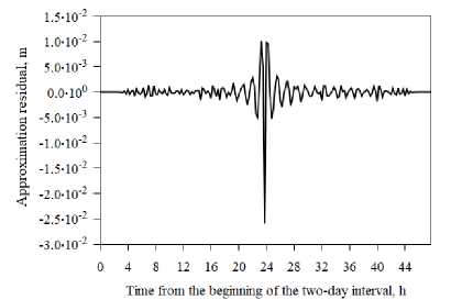
Fig. 3. Approximation residual of the G04 satellite Y coordinate by the 1 00 ^th degree polynomial at the day boundary («ejection») 22–23 May 2016 by the IAC PNT

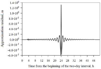
Fig. 4. Approximation residual of the G01 satellite Y coordinate by the 1 00 ^th degree polynomial at the day boundary («ejection») 7–8 November 2016 by the IAC PNT

Рис. 4. Невязка аппроксимации полиномом степени 100 координаты Y спутника G01 на стыке суток («выброс») 7–8 ноября 2016 г. ИАЦ КВНО

Рис. 3. Невязка аппроксимации полиномом степени 100 координаты Y спутника G04 на стыке суток («выброс») 22–23 мая 2016 г. ИАЦ КВНО

In addition to "jumps", "ejections" were also observed in the final orbits of the GPS satellites.

Figures 3 and 4 show “ejections” in the final orbits of GPS satellites G01 and G04, respectively (to be more exact, the effect of “ejections” on the approximation residuals).

The magnitude of the "ejection" in the orbit of the G04 satellite (Fig. 3) determined from the approximation residual is approximately 3.5 cm. In the orbit of the G01 satellite (Fig. 4) the magnitude of the "ejection" is approximately 1.8 m.

The next anomaly that this technique can detect is the behavior of the final orbit of the navigation satellite when performing a maneuver. It is possible to confirm the presence of the GPS satellite’s maneuver using NANU messages (Notice Advisory to Navstar Users) [12; 13]. The satellite G15, according to NANU reports, performed one of the maneuvers on August 20, 2013. Let us consider the approximation residual of X coordinate of this satellite’s final orbit by the 100th degree polynomial for August 20–21, 2013 (Fig. 5).

According to NANU, the satellite maneuver began at 13:01 GPS Time and ended at 19:42 GPS Time. From the timing diagram of the residual in Fig. 3 it can be seen that in the middle of this section there is a peak in the residual of the satellite orbit approximation. We note the difference in the shape (stretching along the time axis) of the residual anomalies for Fig. 3-5.

On the basis of the residuals of the approximation results it is possible to determine the areas of entering the shadow, the time diagram of the residual for such a situation is shown in Fig. 6. To confirm entering the shadow, the SOE angle (Sun - Object - Earth) which corresponded to the presence of shadow parts of the orbit in this time interval was determined.

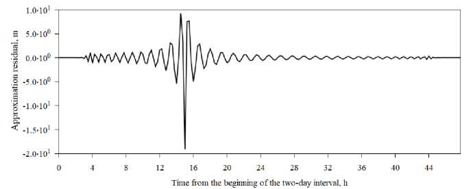
Fig. 5. Approximation residual of the G15 satellite X coordinate by the 100th degree polynomial at the day boundary 20–21 August 2013 by the IAC PNT

Рис. 5. Невязка аппроксимации полиномом степени 100 «маневра» координата X спутника G15 на стыке суток 20–21 августа 2013 г. ИАЦ КВНО

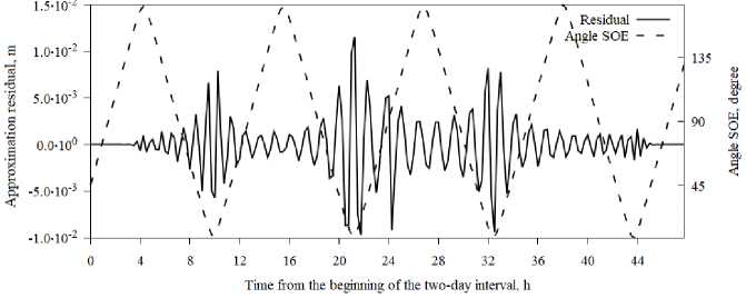
Fig. 6. The time diagrams of the approximation residual for the satellite R03 for the time interval 30–31 May 2013

Рис. 6. Временные диаграммы невязки аппроксимации для спутника R03 для временного интервала 30–31 мая 2013 г.

In the future, when accumulating statistics of anomalies at various analytical centers, we will consider the maximum of the residual modulus (for each satellite, the maximum value of three coordinates is taken).

Anomaly statistics in final GPS orbits

In [7], statistics of anomalies in the final orbits of various analytical centers for GLONASS satellites is given. This section shows anomaly statistics for GPS satellites from 2010 to 2018.

We divide the found maxima of the residual modulus (in all three coordinates) into 2 groups: less than 10 and more than 10 cm.

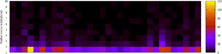
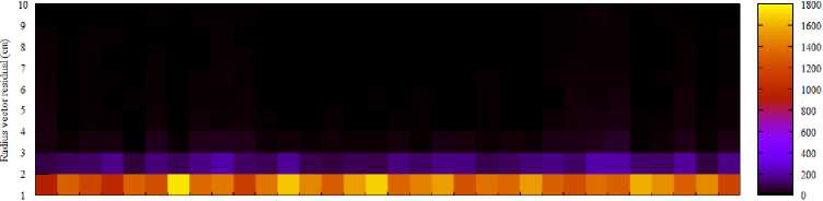
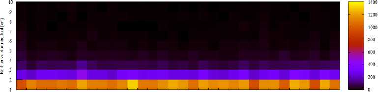
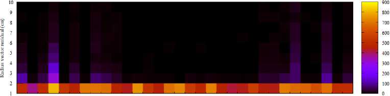
For the group where the value is less than 10 cm, we construct a two-dimensional distribution, where we choose the satellite to which the maximum of the residual modulus belongs at each two-day interval (the interval starts at the beginning of each day) as one of the measurements, and the value of this maximum residual modulus with a step of 1 cm - as the second measurement. The accumulation of the number of anomalies is performed over the entire time interval (from 2010 to 2018), for each analytical center graphs are plotted separately. Two-dimensional histograms for each analytical center are shown: in fig. 7 for CODE, in fig. 8 for ESA, in fig. 9 for IAC PNT, in fig. 10 for IGS. To the right of the histogram there is the legend of the number of anomalies from 2010 to 2018.

For the group of less than 10 cm, it can be noted that the final orbits of different analytical centers have a different number of anomalies exceeding 1 cm. The CODE Analytical Center has no more than 120 anomalies per satellite in the range from 1 to 2 cm. The ESA Analytical Center has on average from 1500 to 1800 anomalies in the range from 1 to 2 cm for each satellite. The analytical center of the IAC PNT has an average of 1000 to 1400 anomalies in the range from 1 to 2 cm for each satellite. The IGS analytical center has an average of 400 to 900 anomalies ranging from 1 to 2 cm per satellite. In this regard one can see the relationship in the number of anomalies per satellite between the CODE and IGS analytical centers.

There are significantly fewer situations when the maximum of the residual modulus exceeds the threshold of 10 cm; for such situations, we also construct a two-dimensional distribution. We choose a satellite as one of the measurements, and the beginning of the annual interval (with a step of 1 year) as the second measurement. For each year, the number of anomalies with a maximum residual modulus of more than 10 cm is accumulated at all two-day intervals of approximation, for each analytical center separately. The resulting distributions are shown in Fig. 11 for CODE, 12 - ESA, 13 - IAC PNT, 14 - IGS. The legend of the number of events is shown to the right of the histogram.

The most significant anomalies of a massive nature (for almost all NSs) were observed at the IAC PNT analytical center in 2014 and 2016. For different analytical centers, it can be noted that there were years when, for certain satellites, the maximum number of anomalies per year was reached for a given center. Moreover, such situations are not always interconnected at different centers. This is partly explained, among other things, by gaps in the SP3 data published by each center (when the center did not lay out orbits that were unreliable from its point of view): the day with large anomalies for one center could have simply been thrown out by another center and are not present thereby in the statistics in Fig. 11-14. Availability (availability on IGS servers) of SP3 data for the CODE analytical center is 97%, for ESA - 90%, for IAC PNT -93%, and for IGS - 95%. On average, for all analytical centers, the maximum number of anomalies exceeding 10 cm is no more than 20.

GO! GO2 GO3 GO4 GOS GO6 GO7 GOS GO9 GIO Gil G12 G13 G14 G15 G16 G17 G1S G19 G20 G21 G22 G23 G24 G25 G26 G27 G2S G29 G30 G31 G32

Satellite

Fig. 7. Distribution of the number of anomalies of less than 10 cm over the observation interval

from 2010 to 2018 for the CODE analytical center

Рис. 7. Распределение количества аномалий менее 10 см за интервал наблюдения с 2010 по 2018 гг. для аналитического центра CODE

G01 G02 GO3 G04 GOS GO6 GOT GOS GO9 GIO Gil G12 G13 GU G15 G16 G17 G1S G19 G20 G21 G22 G23 G24 G25 G26 G27 G2S G29 G30 G31 G32 Satellite

Fig. 8. Distribution of the number of anomalies of less than 10 cm over the observation interval from 2010 to 2018 for the ESA analytical center

Рис. 8. Распределение количества аномалии менее 10 см за интервал наблюдения с 2010 по 2018 гг. для аналитического центра ESA

GO1 GO2 GO3 G04 GOS GO6 GO7 GOS GO9 GIO GU G12 G13 GU G15 G16 G17 G1S G19 G20 G21 G22 G23 G24 G25 G26 G27 G2S G29 G3O G31 G32

Satellite

Fig. 9. Distribution of the number of anomalies of less than 10 cm over the observation interval from 2010 to 2018 for the IAC PNT analytical center

Рис. 9. Распределение количества аномалии менее 10 см за интервал наблюдения с 2010 по 2018 гг. для аналитического центра ИАЦ

GO1 GO2 GO3 GO4 GOS GO6 GO7 GOS GO9 GIO Gil G12 G13 GU G15 G16 G17 CIS G19 G20 G21 G22 G23 G24 G25 G26 G27 G2S G29 G3O G31 G32

Satellite

Fig. 10. Distribution of the number of anomalies of less than 10 cm over the observation interval

from 2010 to 2018 for the IGS analytical center

Рис. 10. Распределение количества аномалии менее 10 см за интервал наблюдения с 2010 по 2018 гг. для аналитического центра IGS

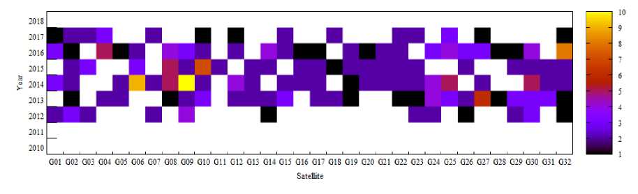
Fig. 11. Distribution of anomalies over 10 cm by year for the CODE analytical center

Рис. 11. Распределение аномалий более 10 см по годам для аналитического центра CODE

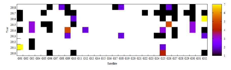
Fig. 12. Distribution of anomalies over 10 cm by year for the ESA analytical center

Рис. 12. Распределение аномалий более 10 см по годам для аналитического центра ESA

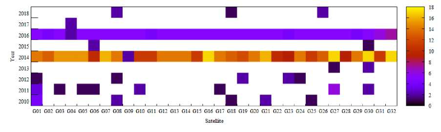
Fig. 13. Distribution of anomalies over 10 cm by years for the IAC PNT analytical center

Рис. 13. Распределение аномалий более 10 см по годам для аналитического центра ИАЦ

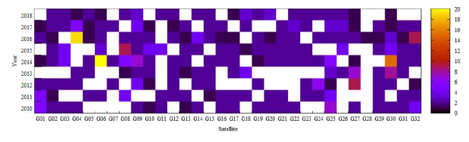
Fig. 14. Distribution of anomalies over 10 cm by year for the IGS analytical center

Рис. 14. Распределение аномалий более 10 см по годам для аналитического центра IGS

The position of the maximum of the residual modulus in the approximation window was analyzed. Most often, the maximum occurred at the boundaries of daily intervals, however, for GPS satellites there were situations when the anomaly did not occur at the boundary of daily intervals, which was almost always associated with the maneuvers of GPS satellites.

As it can be seen from the histograms, all analytical centers have both large (more than 10 cm) and small (less than 10 cm) anomalies in the final orbits, which, nevertheless, are proposed to be used in high-precision positioning problems.

Anomalies detected in GPS satellites clock drifts

For two-day intervals at the end of the day, for which anomalies in the maximum of the residual modulus exceeding several cm were observed (for different analytical centers, different minimum deviations were chosen), the clock drifts with the removal of the linear (and quadratic for large time intervals) trend were investigated.

For the period from 2010 to 2018 statistics of discontinuities whose magnitude in the radius vector exceeded 5 cm was accumulated. For GPS satellites in the data of the CODE analytical center there were 42 such situations. In the data of the IGS analytical center there were 275 of them, while situations were excluded when the discontinuity in the radius vector exceeded 10 cm. At the boundaries of the day with a discontinuity in the orbit, the satellite clock drifts were approximated by a linear function and the approximation residual was calculated. Further, a joint analysis of the residuals of the orbit approximation and the clock drift of this NS was carried out. As it turned out, when solving the PPP problem, these residuals (data discontinuities), as a rule, cancel each other out. A typical example of compensation for discontinuities at the boundary of the day in orbit and clock drift is shown in Fig. 15, 16.

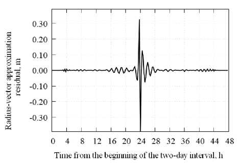
Fig. 15. Radius-vector distance approximation residual by the 100th degree polynomial of the G30 satellite at the day boundary 30 November 2010 – 01 December 2010 by the CODE

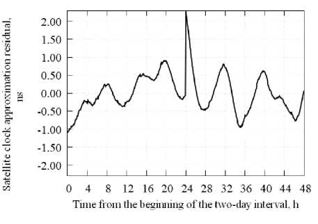
Fig. 16. Clock drift approximation residual of the G30 satellite by the 1st degree polynomial at the day boundary 30 November 2010 – 01 December 2010 by the CODE

Рис. 15. Невязка аппроксимации расстояния по радиус-вектору полиномом степени 100 орбиты спутника G30 на стыке суток 30 ноября – 1 декабря 2015 г., центр CODE

Рис. 16. Невязка аппроксимации ухода часов спутника G30 полиномом степени 1 на стыке суток 30 ноября – 1 декабря 2015 г., центр CODE

In fig. 13 the discontinuity in the orbit along the radius vector is about 60 cm; in solving PPP problems it is partially compensated for by a time gap (about 2 ns).

Influence of anomalies in IGS products on solving the PPP problem

The problem of high-precision positioning (PPP) is to find the coordinates of the station with centimetric accuracy and its clock drift from direct measurements of the phase and pseudo-range from the NS signals. To solve this problem, it is necessary to use high-precision ephemeris and a posteriori estimates of the NS clock drift, which we take from the final SP3 and RINEX Clock files of the IGS service, as well as other processing centers. Besides, according to [14], to achieve adequate accuracy it is necessary to take into account the following effects:

– relativistic clock correction [15];

– signal delay in the troposphere (when performing this work, the model from [15] is used, the formula (9.12), while the parameters D hz , D wz , G N , G E are modeled using a piecewise linear function, the values of the functions at the nodes are estimated together with the coordinates and station clock drift);

• -    displacement of the phase center of the NS and station antennas, as well as the variation of the phase center depending on the angle at which the signal is transmitted and received with respect to the nadir and zenith, respectively (these corrections are transmitted in ANTEX files by the IGS service);

• -    correction for the rotation of the signal phase when turning the NS relative to the receiver;

• -    displacement of the ground measuring point due to deformations of the earth's crust caused by tides in the solid body of the Earth, uneven rotation of the Earth, as well as the pressure of oceanic water moving under the action of the tidal forces of the Moon and the Sun [15].

The initial data in the PPP problem are pseudo-range and phase measurements according to NS signals. The estimated parameters are station coordinates, receiver clock drift, tropospheric signal delay model parameters, and phase ambiguity. A measurement data model is a system of conditional equations linking measured and estimated quantities. The system is solved by linearization according to the specified parameters; the linear system is solved by the least squares method.

In this work we used measurement data from IGS stations [1]: KOKV, MGUE, MAD2, and HRAO. For such stations, the days were chosen when the satellite with an anomaly in orbit was in the radio visibility zone of the station at the boundary of the day (anomalies were determined by polynomial approximation). Two series of experiments were carried out in which parameters such as the pseudo-range residual between the measured non-ionospheric combination and the one modeled in the PPP problem as well as the coordinates of the observation station were estimated.

In the first series of experiments, the PPP problem was solved at two-day intervals with an anomaly in the orbit of a satellite at the boundary of these intervals. In the experiments the influence of the anomaly in the satellite's orbit on the residuals between the measured non-ionospheric phase pseudorange and its model value was estimated first of all. In the residuals, anomalous "jumps" were observed, both for the satellite with an anomaly in its orbit and for other satellites. At the next stage of this series of experiments we excluded satellites with an anomaly in the orbit from the solution of the PPP problem. After that, the residuals of the pseudorange were analyzed again. As a result, the anomalies in the pseudo-ranges near the boundary of the day decreased their value or completely disappeared. At the third stage of this series of experiments, instead of excluding the satellite with an anomaly in its orbit, we tried to “correct” this anomaly by forming a new orbit using the satellite motion model described in the IERS Conventions [15], matching it with the published final orbits on a two-day interval. The analysis of the pseudo-range residuals showed that orbits corrected in such a way not only do not reduce the magnitude of the "jump" or "ejection" of the residuals, but often lead to their increase. This situation is a consequence of the fact that satellite clock drifts also contain anomalies, and these anomalies often compensate for anomalies in orbits, therefore, an approach related to correcting only anomalies in orbits cannot be applied.

The second series of experiments was devoted to assessing the quality of the PPP problem solution on a relatively small interval, which is located at the boundary of the day with the anomaly. In the experiments an interval of 2 hours before and after the boundary of the day (Fig. 17) was considered, during which the PPP problem was solved.

point in time at PPP is solved

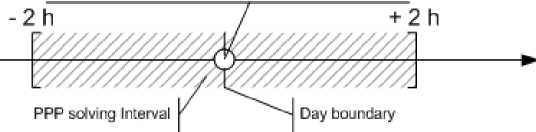
Fig. 17. Timing diagram of solving the PPP problem in the second series of experiments

Рис. 17. Временная диаграмма решения задачи PPP во второй серии экспериментов

Thus, the PPP problem was solved in three versions: a) satellites with an anomaly in orbit were included in the solution; b) satellites with an anomaly were excluded from the solution; c) for satellites with an anomaly the orbit was corrected. The station coordinates obtained by averaging three solutions of the PPP problem were taken as the reference coordinates over a two-day interval: at the beginning, in the middle, and at the end. As a result, it was revealed that in most cases excluding a satellite with an anomaly in its orbit from the PPP solution reduces the error in determining the coordinates. Attempts to "correct" the satellite's orbit with an anomaly in it only increase the error in determining the coordinates.

The Euclidean norm of the distance between three averaged coordinates and three coordinates determined in solving the PPP problem was also determined to assess the quality of solving the PPP problem in this series of experiments. Their statistics for all stations at all solution intervals are shown in the table.

Euclidean distance norm distribution statistics between averaged and determined coordinates

	Without anomalous satellites	With anomalous satellites	Orbit correction was carried out for anomalous satellites
Maximum	151 cm	115 cm	28088 cm
Mean	37 cm	36 cm	2682 cm
RMSD	26 cm	21 cm	3407 cm

As it can be seen from the table, the solution without satellites with orbital anomaly is on average 1 cm worse than the solution with the anomalous satellite, while the solution with the corrected orbit is on average 2682 cm worse.

Conclusion

In the ephemeris and clock products of GNSS analytical centers there are often significant anomalies at the boundaries of the day, which negatively affects the accuracy of solving navigation problems. We proposed and tested on a 9-year time interval a simple technique for finding discontinuities and other anomalies in the final orbits published by the IGS analytical centers. The above analysis of the anomalies showed that there is a mutual compensation of discontinuities in the orbit and the drift of the satellite clock when solving PPP problems. Attempts to "correct" the orbits in order to remove discontinuities at the boundary of the day do not make sense without a corresponding correction of the NS clock drift, which is not possible at this stage.