Application of an integrated support vector regression method in prediction of financial returns

Published Online June 2011 in MECS

The ability of accurately predicting financial returns is invaluable for financial institutions. Reliability predictions are used for various purposes, such as reliability assessment, evaluating risks and liabilities, evaluating replacement policies etc. Thus numerous models have been depicted to provide the investors with more precise predictions. Unlike traditional statistical models, SVM is data-driven, non-parametric model and let ”the date speak for themselves”. Recently, with the introduction of Vapnik’s ε—insensitive loss function, SVM has been extended to solve nonlinear regression estimation problems and has been used successfully to solve forecasting problem in various fields. At present, SVR has been used in predicted areas widely. It’s not easy to judge whether financial returns is purely linear or nonlinear due to the complexity of financial returns. Therefore, many empirical results have indicated that combination of different is able to increase the forecasting accuracy as well as improve the robustness of forecasting models. In this article, the linear and nonlinear SVM models are combined to capture the data pattern of financial returns.

Several studies have proved that the SVM is capable to correctly predict, but there remains two problems for the SVM, namely feature selection and optimal SVM parameters setting , which influence each other, that means that they should be dealt with at the same time.

Therefore, an integrated Support Vector Regression model is built to overcome the problem. In the new model feature selection and SVM parameter optimization are considered simultaneously.

Genetic algorithm(GA) is used for the feature selection and chaotic particle swarm optimization algorithm(CPSO) is used for parameter optimization. A series of experiments show that the proposed GA-CPSO-SVR possesses better ability of finding the global optimum compared with other methods. More detail of the proposed model is presented in Section II.

• II.    A integrated Support Vector Regression (GA-CPSO-SVR)

Bell Laboratories by Vapnik and co-works, as a new machine learning method, has been very successful in pattern classification and regression problems for crisp data [3].

• A.    Support Vector Regression(SVR)

The basic concept of the SVR is to map nonlinearly the original data x into a higher dimensional feature space. Hence, suppose we are given a training data set {( x ₁, y ₁),( x ₂, y ₂),...,( x_n , y_n )} ⊂ N * R , where N denotes the space of input patterns—for instance, R_k .

In ε —SVM Regression, the goal is to find a regression function f(x):that has at most ε deviation from the actually obtained targets y_i for all the training data. In other words, we do not care about error as long as they are less than ε , but will not accept any deviation larger than ε . An ε — insensitive loss function

L ξ ( x , y , f ( x )) = { 0 ^{y - f ( x )} else (1)

so the error is penalized only if it is outside the ε—tube . Fig.1 depicts this situation graphically. To make the SVM regression nonlinear, this could be achieved by simply mapping the training patterns xi by a nonlinear transform φ: N→F into some high dimensional feature space F. A simple example of the nonlinear transform φ is the polynomial transform function:

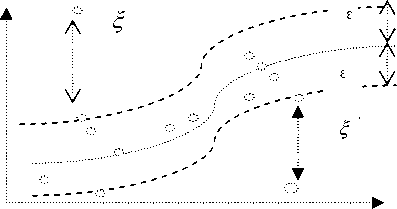
Figure 1. The epsilon insensitive loss setting corresponds for a linear Support Vector regression machine x=(x1, x2) →φ(x) =(у/3x1, 3x2, 3x12, 3x22, 6x1x2, 3x12x2, V3x1x22, x13,x23)                                                                            (2)

Where the degree of the polynomial transform function is 3, and dimension is input space N and feature space F is 2 and 9, respectively. A best fitting function f ( x ) = ∑ ^N w_i ϕ _i ( x ) + b = w^T ϕ ( x ) + b                          (3)

i = 1

where

ϕ _i ( x ) is the feature of inputs x; both w _i and b are coefficients which are estimated by minimizing the regularized risk function:

To avoid over-fitting in the very high-dimension feature space, one should add a capacity control term, which in the SVM case results to be ||w||2. Formally, the SVM regression model can be written as a convex optimization problem by requiring:

ε-tubeMinimize: R(w,ζ,ζ*) =1 w2 +C(∑N (ζi+ζi*))

With the constraints:

w_i φ ( x_i ) + b - d_i ≤ ε + ζ _i ^* , i = 1,2,..., N ,

- w_i φ ( x_i ) - b + d_i ≤ ε + ζ _i , i = 1,2,..., N ,

ζi,ζi*≥0,i=1,2,,

The constant C>0 determines the trade off between the complexity of f(x) and the amount up to which deviations larger than ε are tolerated. We can estimate a linear function in the feature space that makes SVM regression attractive. In addition, the regression task was achieved by solving a convex programming with linear constraints that means it has a unique solution. The size of ε — insensitive is a pre-defined constant. The modeling performance may seriously affected by the selection of a parameter. The ε — insensitive zone represented as a tube shape in the SVM regression, only the training data outside the ε —tube will be penalized. In many real-world applications, the effects of the training points are different. We would require that the precise training points must be regressed correctly, and would allow more errors on imprecise training points.

The constrained optimization problem in (4) is solved using the following primal Lagrangian form:

∑ ^l | a_i - p_i |

Min f = MAPE         =i=1 ii*100% cross validation

Karush-Kuhn-Tucker (KKT) conditions are applied to the regression, and (4) thus yields the dual Lagrangian, J(ai,ai*)=∑Ndi(ai-ai*)-ε∑N(ai+ai*)-1 ∑N∑N(aj-a*j)K(x,xi)

i = 1 i = 1 2 i = 1 j = 1

s.t.

∑ ^N ( a i - a i *) = 0, 0 ≤ a i , a i ^* ≤ C , i = 1,2,..., N .

i = 1

Both α _i and α _i ^* are called Lagrangian multipliers that satisfy the equalities α _{i *} α _i ^* = 0 .

Hence an optimal desired weights vector of the regression hyper-plane is represented as N

w * = ∑ ( α _i - α _i ^* ) K ( x i , x j ) i = 1

Therefore, the regression function could be f ( x , α , α *) = ∑ ^N ( α i - α i ^* ) K ( x i , x j ) + b i = 1

Here, K ( x i , x j ) is called the kernel function. The value of the kernel equals the inner product of two vectors x i and x j in the feature ϕ ( x_i ) and ϕ ( x_j ) ; that is K ( x_i , x_j ) = ϕ ( x_i ) * ϕ ( x_j ) . Any function that satisfies Mercer’s Condition by Vapink can be called the Kernel function.

There are several frequently-used kernel functions, all of them have their own advantages and disadvantages.

In this work, the linear kernel function, represented as (9), is employed for linear SVM model.

K ( x_i , x_j ) = x_i^Tx_j                                                      (9)

In general , a mixed kernel function is used for nonlinear SVM model. With the purpose of better learning ability and better generalization ability. In order to here a global kernel and a local kernel are combined to achieve a mixed kernel function. For instance , we usual use addition, multiplication to combine two or more kernels. For instance, there are two kernels k ₁ and k ₂ that we can possible define a kernel k = k ₁ + k ₂ .Given a set of kernel k = { k ₁, k ₂,..., K_m } , in this article, the linear combination can be represented as :

m k=∑uiki                                               (10)

i = 1

For example, the Gaussian function and the linear function are mixed with a specified weight m, shown as (11)

K ( x_i , x_j ) = m exp( ^{- || x i -} ₂ ^{x j ||} ) + (1 - m ) x_i ^T x_j              (11)

2 σ

The selection of the three parameters ( σ , ε , c ) of a SVM model is important to the accuracy of forecasting. Notably, there are only two parameters, ε and c , for the linear SVM model. However, structural methods for confirming efficiently the selection of parameters efficiently are lacking. Therefore, CPSO is used in the proposed SVM model to optimize parameter selection.

• B.    Genetic algorithm for the feature selection

Genetic algorithm(GA), proposed by Holland, which is an organized random search technique and which imitates the biological evolution process. The algorithms try to retain genetic information form generation to generation that are based on the principle of the survival of the fittest. GA has been successfully applied to a series of problems such as data mining and optimization. It has also been used for the feature selection in SVM modeling[4].

As to a specific problem, The GA looks a solution as an individual chromosome. It defines an initial population of these individuals, which represent the solution space of the problem. First a set of chromosomes is randomly chosen from the search space to form the initial population. Second the individuals are selected in a competitive manner, based on their fitness as measured by a specific objective function. The chromosome are binary-encoded, each bit of the chromosome represents a gene.

In our implementation of GA, a binary string with each bit representing a feature(‘1’ means that this gene is kept in the gene subset and ‘0’ represents the gene is not included in the subset)was used to represent a chromosome. The GA is then applied to a population of randomly generated binary stings. The fitness of each string is determined as follows:

fitness = W A * SVM _ accuracy + W F * N F                      (12)

Where W_A is the SVM classification accuracy weight, N_F is the number of feature selected, W_F is the weight of feature number. The accuracy of 10-fold cross validation was used as SVM _ accuracy .

W_A and W_F both can be adjusted based on their relative importance.

The Genetic algorithm for the feature selection is presented as follows.

• •    Step 1: (Initialization): In this study, the initial population was composed of 50 randomly created chromosomes. The population size of 50 was selected as a trade-off between the convergence time and the population diversity.

• •    Step 2: (Fitness evaluation): Evaluate the fitness of each chromosome. The fitness value for each chromosome was calculated according to

V l. I a i - p i |

-^Min f MAPE^ validation         ^a _l ^{i p i |} *100% (13)

Where l is the number of training data samples; ai is the actual value, and pi is the predicted value. The solution with a smaller MAPE s validation of cross the training data set has a smaller fitness value, and thus has a better chance of surviving in the successive generations.

• •    Step 3: Selection: A standard roulette wheel was employed to select 10 chromosomes from the current population

• •    Step 4: Crossover. The simulated binary crossover (Deb & Agrawal), 1995; Deb & Kumar, 1995)

was applied to randomly paired chromosomes. The probability of creating new chromosomes in each pair was set to 0.7. The newly created chromosomes constituted a new population.

• •    Step 5: Mutation: The mutation operation follows the crossover operation and determines whether a chromosome should be mutated in the next generation. This study applied polynomial mutation methods to the proposed model. Each chromosome in the new population was subject to mutation with a probability of 0.08.

• •    Step 6: Elitist strategy: The fitness value was calculated for the chromosomes of the new population. If the minimum fitness value of the new population is smaller than that of the old population, then the old chromosome can be replaced with the new chromosome of the minimum fitness value.

• •    Step 7 : Stopping criteria. The process was repeated from 2 to 6 until the number of generations was equal to 60. If the number of generations equals a threshold, then the best chromosomes are presented as a solution; otherwise go back to Step2.

An overview of GA for the feature selection will be given in the next subsequent paragraphs.

The setting probability of parameter is largely effect the converged solution. In this study, the crossover probability is recommended from Holland. The choices of other parameters such as the mutation--probability, population seize are based on numerous experiments as those values provide the smallest MAPE crossvalidation on the training data set.

• C.    CPSO algorithms for selecting parameter of SVR model

In SVR, parameters inappropriately chosen result in over-fitting or under-fitting. Generally, when selecting the parameters, most researchers still follow standard procedure (trial-and-error).First building a few SVR models based on different parameter sets, then testing them on validation set to obtain optimal parameters. However, this procedure is time-consuming and requires some luck.

Particle swarm optimization(PSO), for easy implementation and quick convergence, has gained much attention and wide applications in solving continuous nonlinear optimization problem. Particle swarm optimization system begins with the random initialization of a population and multiple candidate solutions in the problem search space. Each particle looks for the optimal position to land. Finally the best global position can be attained by adjusting the direction of each particle towards its own best location at each generation. Adjust the velocity of each particle to improve the direction of each particle,tracking and memorizing the best position encountered could cumulate each particle’s experience. So each particle remembers the best position where it reached in the past, then the PSO system combines local search method with global search methods.

In a SVR model, the velocity, the position, the best position of each particle, due to the three parameters, that can be represented as (14)-(16)

xk (I) = [ x(k ) i ,1, x(k ) I ,2,... x(k ) I, n ], vk (I) = [ v (k ) i ,1, v(k ) i ,2,.-. v(k ) i, n ],

P k ( i ) = ^[ P ( k ) . ,1 ^, P ( k ) . ,2 ^, ... P ( k ),, n L                                                    ⁽¹⁶⁾

k = c , s , a , i = 1,2,.... N

Thus the global best position among all particles in the swarm x_k = [ x _{( k }1}, x _{( k )2},... x _{( k} ) _N ] is computed by (12)

Where l and l are the maximum and minimum of l, max min respectively, fi is the current objective value of the particle, favg and fmin are the average and minimum objective values of all particle , respectively.

CLS is used to perform locally oriented search for the solution f_globali , which is resulted from PSO. CLS is based on the logistic equation, with sensitive dependence on initial conditions, and is defined by the following equation:

cx ( - ¹ ) = 4 cx "(1 - cx ‘ k „) ⁽²¹⁾

p ( k ) global    ^[ P ( k ) g ,1 , P ( k ) g ,2 ,... P ( k ) g , d ^]

The new position of each particle in next generation can be shown as (18)

^V ( k )4 t + ¹⁾ = ^lV ( k ) . ⁽ t ) + m 1 r^a”^{d (1)( P} (k ) . - x ( k ) . ( t > ) + m 2 r^a”^{d (2)( P} ( k ) g

k = c , s , а , i = 1,2,..., N

Where cx _{( k} ) i is the i _th chaotic variable; X represents the iteration number, cx ₍ ⁽ X ₎ ⁾ _i is distributed in the range(0,1) (0)                        (0)

and cx ( k ) i fc (0,1) but cx ( k ) i ^c {0.25,0.5,0.75} -

The procedure of CLS is illustrated is presented as follows:

Where l is called the inertia weight that controls the impact of the previous velocity of the particle on its current one, m ₁ and m ₂ are called acceleration coefficients.

Step 1: Setting X = 0 and map the three parameters into chaotic variable

X _ x(k )i   x min( k ) i cx (k) i = x max( k ) i — xmin( k ) i

After the velocity has been updated, the new position of the particle for each parameter in the next generation is shown as(19)

Step 2: Compute the next iteration chaotic variable cx X ⁽ i + ¹⁾with (16).

( k ) i

X_tk ) , ( t + 1) == V ( k ) . ( t + 1) + X ( k ) , ( t )

X = [ X 1 , X 2 ,..., X n ]

Step 3: Obtain three parameters for the next iteration by the 17 and compute the new objective value

x ( k ) i ⁾ = x mn k ) i ⁺ cx k ) i ) ⁽ x mix( k ) i ^x min( k ) i )

Where l is called the inertia weight that controls the impact of the previous velocity of the particle on its current one; m1 and m2 are two positive constants called acceleration coefficients; rand(1) and rand(2) are two independently uniformly distributed random variables with rang^^0,1] V k „-= ^[ V_{k )} 1 ^, V (k ₎ 2 ^,...^, V (k ) n ^] represents the distance to be traveled by the particle from its current position; X = [ X ₁, X ₂,..., X N ] means the position of particle l , and p_{best ( i )} the best previous position of particle l ; p_{gbest ( i )} t represents the best position among all particles in the population.

The performance depends on its parameters in the procedure of PSO, it often lead to be trapped in local optimum. Thus proper control of l is very important to find the optimum solution accurately.

To overcome the problem, a chaotic PSO (CPSO) method that combined PSO with AIWF (adaptive inertia weight factor) and chaotic local search (CLS) is employed to overcome the shortcoming. CPSO is a two phase iterative strategy based on the proposed PSO with AIWF and CLS, in which AIWF is used to encourage good particles to improve the exploration to refine results by local search, and bad ones to modify searching space with large step. AIWF is determined as(20)

• Step 4: If the new objective value with smaller forecasting accuracy index value or maximum iteration is reached, then, the new chaotic variable x ₍ ⁽ X + ¹¹ and its corresponding objective value is the final solution; otherwise, let X = X + 1 and go back to Step 2.

In the investigation, the normalized mean squared error (NMSE), shown as (22), serves as the forecasting accuracy index for identifying suitable parameters, determined in Step 4 of PSO and in Step 5 of CLS, for use in the GA-CPSO- SVR model.

n ²

NMSE = — —_г X ( a . — f. ) n 5

（ 24 ）

1 = ^

( l max

¹ min ⁺

-1

-1 m,n )( f, — fmJ

min

if f, ⁵ f avg

max

else

Where 5 ² = ¹X ” ,( a — a ) 2 and n = ¹

• n is the number of forecasting periods;

• a_i is the actual value at period i ;

• f_i denotes is the forecasting value at period i .

An overview of CPSO parameter settings will be given in the subsequent paragraphs.

Fig. 2 shows the framework of the proposed GA-CPSO-SVR model.

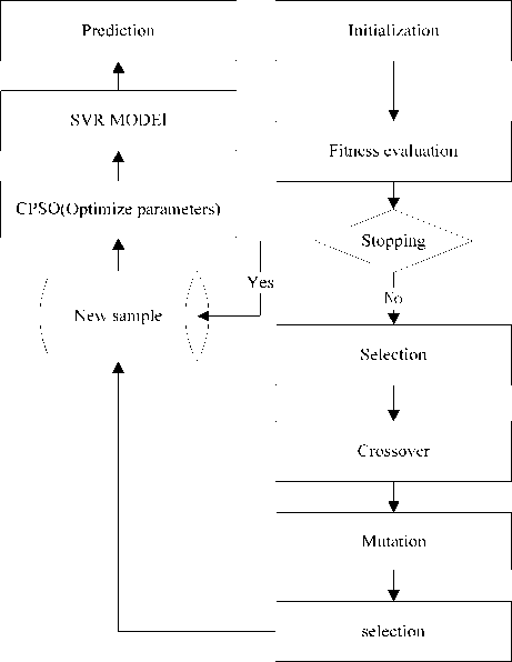
Figure 2. The architecture of a GA-CPSO-SVR model

Notably, N_i ^* is the forecast value of (24). Fig. 3 shows the structure of the GA-CPSO-SVR model proposed in this article.

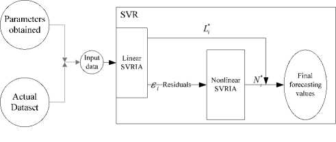
Figure 3. The architecture of proposed GA-SVR-CPSO model for prediction

III A NUMERICAL EXAMPLE

In order to verify the accuracy of the algorithm we proposed in forecasting financial returns. We predict financial returns of the Shanghai Composite Index. The samples of this paper were collected from Shanghai Stock Exchange from February 5, 2006 to January 28, 2007, a total of 358 observations. The samples were ordered from 1 to 358, and we divided them into 3 groups: The training group (from 1 to 150), the validation group (from 151 to 263), the testing group (264-358)

D The proposed SVRCPSO model

A strategy which has both linear and nonlinear modeling abilities is a good alternative for forecasting financial returns for the complex data pattern of financial returns. In this article, the linear GA-CPSO-SVR model is used as a preprocessor to capture the linear data pattern, while the nonlinear GA-CPSO-SVR model is applied right after the linear GA-CPSO-SVR to forecast the nonlinear data pattern of residuals from the linear GA-CPSO-SVR model. The hybrid model (H ) can be represented as :

After the CPSO was applied to search for the optimal parameter sets, the optimal parameters in the Linear GA-CPSO-SVR model. where c=2.639, £ =13.928, and a ² =2.365 , as shown in Fig. 4.

H i = L i + N

Where Li is the linear part; and Ni represents the nonlinear part of the hybrid model. Both of them are estimated from the data set, L*i is the forecast value of the linear GA-CPSO-SVR model at time i. Let ei represent the residual at time i from the linear GA-CPSO-SVR model; then, e = H- L (26)

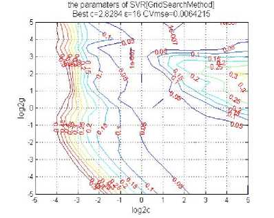
Figure 4. The optimal parameters in the Linear GA-CPSO-SVR model

The residuals are modeled by the nonlinear GA-CPSO-SVR and can be represented as follows:

The parameters of the Nonlinear GA-CPSO-SVR model as Fig. 5 shows

We can see c=2.8284, ε =16 in the Nonlinear GA-CPSO-SVR model.

^e i = ^f < Л - 1 , ^ - 2 ,-, ^e i - n ) ^{+ A} i

（ 27 ）

Where f represents the nonlinear model and A i represents the random error. Thus the combined forecast is

In order to reduce the differences among the different data fractional error. Sample need to be normalized when we have reconstructed the sample. AS the sample which used in this study are all positive. So we shrink them to [0,1] range, data normalization formula is:

__I

X,=

i

min

L * + N * = H

X max

X min

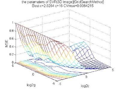
Figure 5. The parameters of the Nonlinear GA-CPSO-SVR model

The results of data after normalization as shown in

Fig. 6:

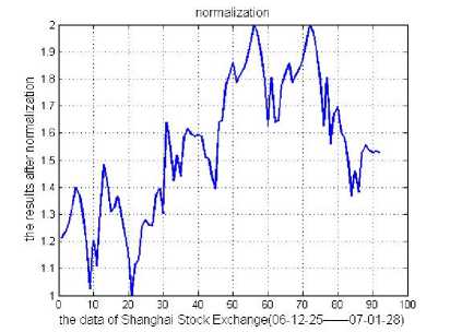
Figure 6 . Data of Shanghai Stock Exchange after normalization

Then the final SVR forecasting models were built. The forecasting simulation was performed against the testing data. Fig. 7 makes comparison of actual values and forecasted values by the proposed model.

In the Fig. 8, we can see the fractional error of actual values and forecasted values with the model we built.

Compare the results obtained with the forecasting results form the Back Propagation Neural Network model (BPNN) and the Auto Regressive Integrated Moving Average model (ARIMA) and Support Vector Regression and CPSO-SVR. Here we use the criterion MAPE (the smallest value of MAPE) to illustrate the accuracy index.

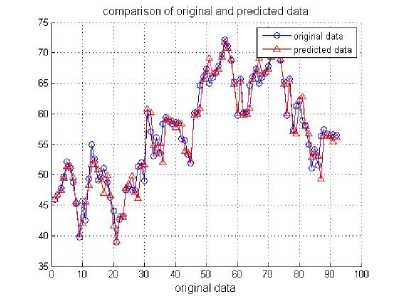
Figure 7. Comparison of actual values and forecasted values by GA-CPSO-SVR model

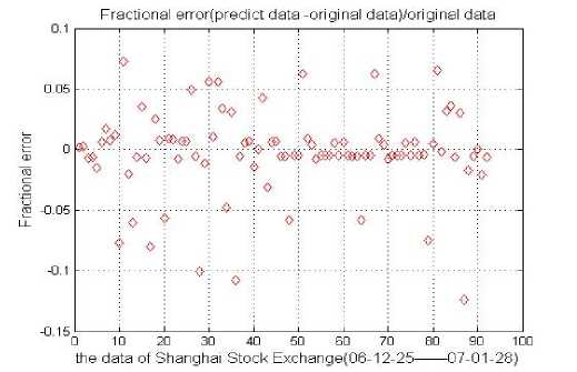
Figure 8. Fractional error of actual values and forecasted values by GA-CPSO-SVR model

TABLE I.     P arameters of HSVRCPSO model

Model	MAPE(%)
GA-CPSO-SVR	3.12
CPSO-SVR	3.69
SVR	4.12
BPNN	4.98
ARIMA	5.64

IV CONCLUSIONS

The motivation of this study is based on the evidence that different forecasting models can complement each other in approximation data sets. This paper applied SVM model composed of linear and nonlinear SVR to the forecasting field of financial returns. Then Genetic algorithm is used for the feature selection in SVR modeling and chaotic particle swarm optimization algorithm is used to search for better combinations three parameters in SVM. Compared with other models, within the forecasting fields of financial returns, the proposed model offers a valid for application in financial market.

However; the algorithm still has to be improved, other advanced searching techniques to determine the suitable parameters should be combined with the SVR model to forecast financial returns. Furthermore the number of input data influences the forecasting performance to a large extent. Thus, to develop a more effective technique available to determine the number of input data will be an important direction for future development.

Acknowledgment