Application of evolutionary algorithms for designing recurrent neural networks in regression problems

The advancement of technological progress is accompanied by a growing number and complexity of tasks in various scientific fields. This requires the development of efficient methods to solve them for ensuring further progress. Currently, there are many algorithms with mathematically proven effectiveness for solving such tasks. However, these algorithms can most often be applied only to well-structured problems with sufficient information about the issue being solved.

In a constantly changing world, having complete information is not always available. This creates a dilemma: either spend a lot of time and resources to study the problem and develop a highly specialized algorithm, or use algorithms that are known to be practically effective. Algorithms of the second type, like neural networks, do not need full information about the problem. They solve it in a way that may not be the most efficient but is sufficient for most situations.

A key disadvantage of neural networks is the high complexity of designing their architecture. To solve this, neural evolution uses Evolutionary Algorithms (EAs) to design the network structure automatically. In EAs, a potential solution is called an individual. One such algorithm is Genetic Programming, where individuals are functions encoded as trees containing functional and terminal nodes.

The terminal nodes correspond to neurons in the input and hidden layers. Functional operators create connections and hidden layers. However, these operators can only create new neurons or add/combine hidden layers. They do not support creating recurrent connections, which could pass useful information from previous iterations. Adding this ability could improve solution quality and expand the space of possible solutions, increasing the algorithm's effectiveness.

The paper is structured with a “Materials and Methods” section describing the regression problem, the algorithms used, and the new proposed operator for creating recurrent connections. The "Numerical Experiments" section tests the algorithm on problems from the Feynman Symbolic Regression Database, comparing it to previous versions using the Wilcoxon rank-sum test (α = 0.05). Hypotheses are formulated to explain the low effectiveness and guide future improvements.

1    Materials and methods1.1    Problem statement

The regression task involves finding a relationship between a set of features (independent variables) and a continuous target variable. Formally, let there be a set of objects (observations) and a set of target (dependent) variables .

It is assumed that there exists an unknown target function (dependency function) that models the relationship between the target variable and the data:

y = f (x), here, x e Rd,X y e R, Y .

The goal of the regression task is to reconstruct the relationship between the target variable and the features using the available data. This goal is achieved by finding a function , called a regression model or algorithm, which maps to . The values produced by this function should be as close as possible to the values of the unknown target function.

Thus, the regression task can be reduced to a minimization problem for the criterion:

¹ E n- 1( y i -ф ( x i ) )2 ^ min, n ¹

here, n is the size of the training sample.

The solution to the problem is a model ф * ( x ) that provides the best approximation of the target variable according to the desired dependency for new data not included in the training sample. The quality of the solution is later evaluated on a test sample using specific evaluation metrics.

1.2    Related work

Neural Networks (NN) can solve classification, regression, and other tasks [1]. A key problem with this method is the high complexity of designing the neural network's architecture, which directly affects the quality of the solution [2].

This problem can be addressed through neuroevolution, which uses Evolutionary Algorithms (EA) for automated architecture design. This approach eliminates the need for a human expert to configure the network, saving significant time and financial resources [3].

In EAs, the mechanism of natural selection is used to find a solution. Each individual, representing a potential solution, is characterized by a numerical fitness value. The higher this value, the better the solution. The fitness value directly influences the probability that an individual will produce offspring and thus participate in forming a new generation. The set of individuals at a specific iteration of the algorithm forms a population. Classical EAs are characterized by the following significant drawback: the complexity of selecting parameters and the combination of algorithm operators (selection, crossover, mutation) for a specific task, since these elements directly affect the quality of the solution. To solve the EA configuration problem, self-configuring evolutionary algorithms (SCEA) are usually applied, whose main advantage over standard analogues is the dynamic adaptation of parameters directly during the problem-solving process [4].

In this work, the approach for automated design of neural network architecture is a SelfConfiguring Genetic Programming (SCGP) algorithm. The used approach encodes individuals in the population using nodes from functional and terminal sets [5]. The following operators of the functional set are used to create a neural network [6; 7]:

• –    Addition (+): the neural network layers to the left and right of the operator are added together and become a new neural network while preserving the old connections.

• –    Concatenation (>): all neurons without outputs connections of the neural network to the left of the operator are connected into all neurons without inputs connections of the neural network to the right.

The terminal set operators used are neurons from the hidden layer, which differ by their activation function, and neurons from the input layer. Decoding an individual, represented as a tree, results in a neural network whose properties are defined by the tree.

A key problem of this automated neural network design method is an absence of predefined rules for building the network in the Genetic Programming algorithm. If the algorithm runs using the chosen operators without additional constraints on the tree structure, even the first individuals will cause many structural conflicts and errors during decoding.

To solve this problem, a specific tree generation scheme was proposed (fig. 1): the root (starting) node is always a union operator; the left subtree can only contain input layer neurons and addition operators, while the right subtree can only contain hidden layer neurons [8].

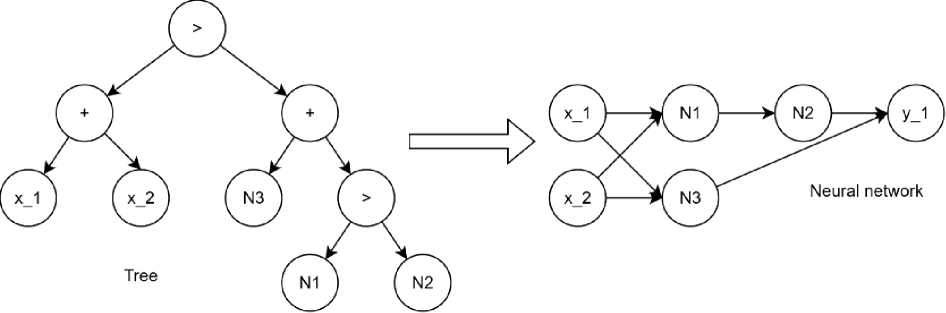
Рис. 1. Пример преобразования дерева в нейронную сеть

• Fig. 1 .    Example transforming tree in neural network

Neural networks often are characterized by the problem of overfitting, where the algorithm learns to memorize the training data instead of identifying general patterns for prediction. To solve this problem, in this paper was used the early-stopping (ES) algorithm [9]. This mechanism stops the weight adjustment process in neural networks with inefficient structures, saving computational resources for investigating more promising architectures.

1.3 Proposed approach

The previous chapter presented an approach for designing neural network architectures using SCGP. However, the proposed functional operators cannot create connections that join neuron outputs in one layer to inputs in the previous (or current) layer. This prevents the design of Recurrent Neural Networks (RNN), which could improve performance on certain tasks (fig. 2). The key feature of RNN is their ability to store information from previous steps in a sequence and use it for processing the current element. This creates recurrent connections that form cycles, allowing information to persist over time [10].

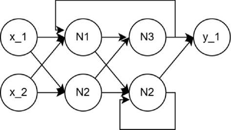
Рис. 2. Пример рекуррентной нейронной сети

• Fig. 2.    Example of RNN

This connection modifies the neuron's formula by introducing additional weights and inputs (when a recurrent connection is present). This increases the complexity of training the neural network, depending on the number of such connections:

S=f (S "=iwi • xi + w + S m=1rj • yj), here f (x) is the activation function, i-.'. is the neuron weight for a regular connection, rj is the neuron weight for a recurrent connection, xi, yj are inputs for regular and recurrent connections, respectively.

The formula used (1) represents one of the ways (and possibly the simplest) to create a recurrent connection, known as short-term memory [11]. One disadvantage of this approach is its inability to retain long data sequences: with each new iteration, information from previous steps decays and gradually has less influence on the next output.

For tasks requiring complete preservation of sequence information (such as in Large Language Models where word order directly affects sentence meaning), this a significant limitation, leading to alternative recurrent connection implementations [12]. However, in regression tasks, this limitation becomes an advantage. When building models, there's no need to know the exact sequence of recent data points, as such information may become irrelevant or contain little useful data (for example, in stock price prediction, early company quotes might not correlate with its current high value). Thus, this limitation is mitigated by the specific application domain of RNN.

If training data is fed into an RNN without preprocessing, the model may make inaccurate predictions due to the nature of short-term memory: information from the most recent iteration has the strongest influence on the neuron compared to all previous iterations. If the data point farthest in the sequence significantly affects the current point, it may harm the iteration by introducing excessive noise. Therefore, all data must be sorted by proximity: the closest points should be positioned near each other in the sequence, enabling each new iteration to benefit from relevant previous information.

To create a functional set operator for SCGP that implements recurrent connections, the following requirements must be considered:

– The recurrent connection can be created for a single neuron (the output of the current neuron is connected to its own input).

– The functional set must allow encoding any solution available in the search space.

Thus, the proposed functional set operator will be unary (to meet the first requirement) and will be used exclusively in the right subtree relative to the root node (to satisfy the second requirement).

In automated neural network design using SCGP, neural masses can emerge the clusters of neurons that have no connections with each other for information exchange (with the exception of the input and output layers) (fig. 3).

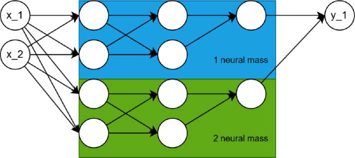
Рис. 3. Пример структуры нейронной массы

• Fig. 3.    Example of neural mass

If such neural masses are detected in the network, it's necessary to choose an approach and establish rules for processing these structures. Several potential solutions exist: creating cross recurrent connections between these neural masses to enable mutual information exchange, thus allowing them to share data for model building. However, this might lead to negative consequences like information overload within these clusters.

Alternatively, a more effective approach could be the opposite: creating connections only within a single neural mass, thereby strengthening its internal information processing while preventing interaction between different masses. Each specific task will have its own optimal solution, and it's impossible to determine this in advance due to the high computational complexity of such preevaluation.

It's most practical to leave this decision to the EA and its evolutionary selection strategy. Through the algorithm's operation, an effective way to process these structures will be naturally discovered.

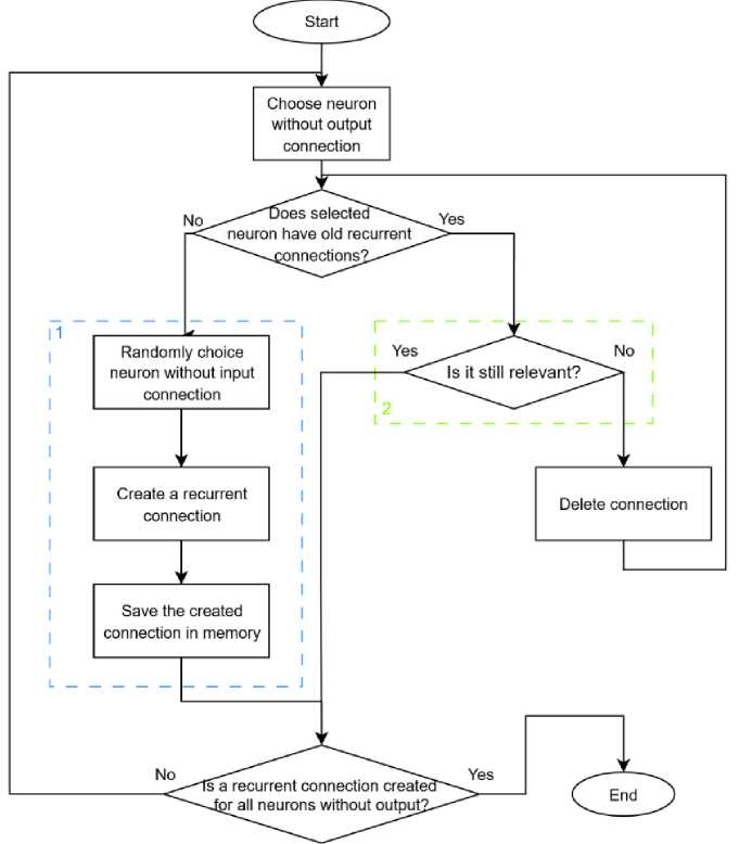
Based on all the above, the unary functional operator will have the following algorithm (fig. 4).

Start

Is it still relevant?

End

Is a recurrent connection Greater Jot all neurons without output?.

^Ijoes selected ^ neuron have old recurrent ■^'-..connections?.-''''’

Yes

Yes

Yes

Save the created connection in memory

Randomly choice neuron without input connection

Create a recurrent connection

Delete connection

Choose neuron without output connection

Рис. 4. Алгоритм создания рекуррентной связи

Fig. 4 . Algorithm for creating the recurrent connections

As shown in the fig. 4, a neuron without standard outgoing connections is first selected. If this neuron has no information about previous recurrent connection (which can be passed through generations), a new connection is created using the following algorithm: a hidden layer neuron without input connections is randomly selected, and a recurrent connection is created. It should be noted that this algorithm also works for a neural network with just one hidden layer neuron.

At the next stage, the created connection is saved. This prevents a complete reset of recurrent connections when the neural network structure undergoes minor changes, which could negatively impact the individual's fitness.

If the individual has a preserved recurrent connection from the past, its relevance is checked. If the connection refers to a neuron that lacks standard incoming connections (as in the previous step), the connection is maintained. If the connection points to a non-existent neuron - meaning the neural network changes were so significant that its structure was completely altered - the recurrent connection is deleted and recreated using the standard algorithm.

2 Numerical Experiments

In this section, experimental setup, results, and discussions are presented. The performance of the algorithm proposed in this paper is evaluated using 12 equations from Feynman Symbolic Regression Database [13]. This database consists 120 equations with different difficulty levels and number of dimensions from one to nine. This equation covers a wide range of physical phenomena.

2.1    The experimental setup

For the research, 12 tasks were selected from the Feynman Symbolic Regression Database, with the following indexes: 1.6.2b, 1.8.14, 1.12.1, 1.12.2, 1.12.4, 1.14.3, 1.14.4, 1.15.3x, 1.15.10, 1.18.4, 1.24.6, 1.34.8. From each task, 1000 points were randomly sampled. The obtained points were divided into training and test sets in a 75 % to 25 % ratio.

The presented modification of the algorithm is an advancement of standard neuro-evolution models, enabling the formation of neural networks. A comparison was conducted with these algorithms to determine the effectiveness of the proposed modification. The comparison will be made between SCGP NN ES and SCGP NN. Also to adjust the weights of neural networks in this paper was used the Differential evolution [14]. This is a global optimization evolutionary algorithm, which don’t used the gradient of error, that’s also solves the problem of vanish and exploding gradients [15].

The stopping criterion for the presented algorithms is reaching a specified number of fitness function evaluations (2,250,000). The fitness function is computed as the inverse of the Root Mean Square Error (RMSE). To study the effectiveness of automated design of recurrent neural networks using SCGP, it is necessary to perform several runs (10) and calculate the average values of the obtained evaluation metrics. This method is used to reduce the influence of the algorithm's stochasticity on the assessment of its effectiveness.

The effectiveness of the algorithms is evaluated using RMSE and the coefficient of determination (R2) based on the best architecture found in each run. The results from all runs are averaged, and the variance is calculated. The algorithm is also evaluated using Wilcoxon’s signed-rank test with a significance level of a = 0.05 .

2.2    Experimental results and discussion

The results of used algorithms are presented in tables 1–5. The first column shows the task number from chosen Feynman Symbolic Regression Database, while another column is represented the results for algorithms in chosen metrics (RMSE, R2).

Table 1

Results of error values for SCGP NN with early-stopping in Feynman Symbolic Regression tasks

№	RMSE mean	RMSE median	RMSE std	RMSE min	R2 mean	R2 std	R2 min
1	0.030255	0.031186	0.001887	0.027186	0.729153	0.033031	0.681566
2	0.798367	0.784630	0.063579	0.722154	0.336326	0.105652	0.182591
3	0.888675	0.784307	0.207547	0.679695	0.963936	0.017017	0.934025
4	0.027339	0.020624	0.013097	0.016995	0.848870	0.152385	0.532484
5	0.007253	0.005990	0.004120	0.005297	0.916750	0.125040	0.541924
6	4.933080	4.489754	1.367572	3.146004	0.935141	0.034235	0.889169
7	1.996298	1.628534	0.786767	1.517677	0.971811	0.024907	0.917305
8	0.204526	0.195591	0.017355	0.187883	0.982622	0.003016	0.977386
9	0.421437	0.440401	0.037056	0.338179	0.959563	0.006617	0.953995
10	0.222793	0.208876	0.026170	0.206589	0.937273	0.015764	0.904050
11	5.709326	6.172551	1.162869	3.028174	0.888363	0.037570	0.850067
12	3.819260	3.771302	0.678411	2.703044	0.819556	0.066333	0.658984

Table 2

Results of error values for SCGP RNN with early-stopping in Feynman Symbolic Regression tasks

№	RMSE mean	RMSE median	RMSE std	RMSE min	R2 mean	R2 std	R2 min
1	0.030967	0.031253	0.001430	0.026945	0.716757	0.024929	0.681324
2	0.768771	0.736520	0.067953	0.694683	0.383719	0.112825	0.122782
3	0.970043	1.017971	0.162875	0.675926	0.958103	0.013062	0.936533
4	0.027461	0.018819	0.013881	0.016239	0.844296	0.159695	0.510323
5	0.008546	0.005866	0.005781	0.004668	0.872636	0.177612	0.512356
6	5.349869	5.800234	1.628757	3.287614	0.922596	0.042573	0.861263
7	2.740801	3.083539	0.884848	1.514471	0.949215	0.028464	0.916276
8	0.275157	0.200556	0.167535	0.189542	0.957194	0.062788	0.775598
9	0.419837	0.430116	0.037056	0.334526	0.959867	0.006739	0.948632
10	0.224578	0.208458	0.029734	0.206547	0.936029	0.018174	0.898910
11	5.752768	6.411327	1.479931	2.517054	0.883970	0.046132	0.843059
12	3.758108	3.701063	0.567414	2.464030	0.826771	0.049829	0.720638

Table 3

Results of error values for SCGPNN in Feynman Symbolic Regression tasks

№	RMSE mean	RMSE median	RMSE std	RMSE min	R2 mean	R2 std	R2 min
1	0.032513	0.031282	0.002389	0.031282	0.686748	0.049288	0.548246
2	0.732702	0.711537	0.044693	0.695596	0.442465	0.070404	0.275806
3	0.897042	0.960038	0.191087	0.604022	0.963573	0.014390	0.946306
4	0.036574	0.032146	0.016772	0.016396	0.733759	0.225528	0.312249
5	0.013806	0.010169	0.008499	0.006038	0.685574	0.346809	–0.00562
6	4.870735	4.183917	1.238393	3.296656	0.937487	0.031304	0.891457
7	1.998499	1.624447	0.769187	1.513158	0.971925	0.024255	0.916692
8	0.203477	0.198328	0.013218	0.187889	0.982851	0.002308	0.977069
9	0.414873	0.420976	0.027051	0.338874	0.960948	0.004734	0.956331
10	0.209917	0.207715	0.004293	0.206619	0.945049	0.002279	0.939507
11	5.889937	6.321806	1.303967	2.748203	0.880329	0.042953	0.833116
12	3.404473	3.441702	0.436398	2.532716	0.858723	0.034825	0.802207

Table 4 presented the comparison of algorithms by using Wilcoxon rank-sum test with the significance level a = 0.05 . To demonstrate what algorithm better, used the special symbols: better (+), worse (–), or not different («=») compared with SCGP RNN with early stopping. The "Results" column shows the counted symbols with followed scheme: better/not different/worse.

Table 4

Wilcoxon rank-sum test results

Vs. SCGP RNN ES

Results

1

2

3

4

5

6

7

8

9

10

11

12

SCGP NN ES

0/12/0

=

=

=

=

=

=

=

=

=

=

=

=

SCGP NN

1/10/1

=

=

=

=

–

=

+

=

=

=

=

=

Table 5

Wilcoxon rank-sum test for another algorithms

Vs. SCGP NN ES     Results      1     2    3    4    5     6    7     8     9     10   11    12

SCGP NN          1/9/2      –    +    =    =   –    =   =    =    =    =    =    =

As can be seen from the Wilcoxon rank-sum test results, the proposed algorithm modification shows no statistical difference from its previous versions. Despite the absence of statistically significant differences compared to previous algorithms, unusual results can be observed in Table 5. In this comparison table with previous versions, SCGPNNES shows statistically better, though only marginally significant, results. This creates an atypical situation where SCGPRNNES demonstrates average performance, positioned between these algorithms without providing either improvements or deteriorations. This anomaly should be investigated to enable future enhancing modifications to SCGPRNNES.

It would be incorrect to evaluate SCGPRNNES based only on the Wilcoxon rank-sum test, as the algorithm might demonstrate better results according to other metrics. Its comparative effectiveness can be analyzed using data from tables 1–3. These tables reveal the following pattern: when considering only numerical values, other algorithms share the best results across different evaluations. SCGPRNNES wins in only a few tasks, which doesn't align with its relatively similar performance in the Wilcoxon rank-sum test.

We can draw the following conclusion: on average, the algorithm showed comparable results according to the Wilcoxon rank-sum test but slightly worse values in Tables 1-3. The key advantage of this modification is its higher probability of finding the best solution for a problem. In most tasks, SCGPRNNES managed to find better solutions that other algorithms couldn't achieve. However, it also produced the worst solutions in most tasks, indicating low stability.

At this stage, it is necessary to determine the reason for SCGP RNN ES's relatively low effectiveness. Several hypotheses can be proposed to explain these results.

The algorithm may have failed to fully leverage the advantage of RNNs due to the absence of suitable tasks. In regression tasks, there is no strict dependence of the result on the sequence of data points. Recurrent connections can introduce useful information but can also overload a neuron, thereby suppressing other inputs. This characteristic might have disrupted neuron tuning because the selected tasks were not designed to search for these sequences. This fact initially placed the algorithm at a disadvantage compared to its counterparts.

The second reason for the algorithm's relatively low results could be the accumulation rate of values in the neuron due to randomly generated weights in the recurrent connection. Such circumstances can directly impact an individual's fitness. As a result, the neural network might end up with zero fitness because the error was too large due to randomness. This problem could be solved by implementing the following mechanism: if a connection comes from a neuron whose activation function returns large values, then this signal should be dampened. This mechanism could protect the neuron from sharp recurrent spikes. An additional requirement would be to initialize low weights for such connections so that the primary information is carried by the standard inputs. Previous versions of the algorithm did not have this drawback due to lesser influence of random factors.

2.3    Conclusion

Based on the research results, the following conclusions can be drawn. The proposed modification, according to the Wilcoxon rank-sum test with a significance level of a = 0.05 , demonstrated no significant improvements. This indicates the need to analyze results using other evaluation metrics, as the algorithm might have shown better performance in them. When examining the numerical values from Tables 1-3, it is evident that SCGP RNN ES finds best solution of the problem in big part of the tasks, but also finds the worst solutions in the same tasks. These findings indicate the relatively low effectiveness of the presented algorithm.

The following proposed hypotheses can explain the reasons for such unsatisfactory results. The tasks used in the study were initially not designed for RNNs, which placed the algorithm at an inherent disadvantage compared to previous versions. The second hypothesis concerns the strong influence of recurrent connections on neurons. The weights generated for such connections might have overwhelmed useful information coming from regular connections. A solution to the latter problem is controlling the initialization of weights for recurrent connections to protect the neuron from their destabilizing influence.

Acknowledgment. This research was supported by the Russian Science Foundation (project № 25-19-20154, , and the Krasnoyarsk Regional Science Foundation.