Application of Krill Herd and Water Cycle Algorithms on Dynamic Economic Load Dispatch Problem

Published Online August 2014 in MECS

Your goal is to simulate the usual appearance of papers Dynamic economic dispatch (DED) is one of the most principal and serious issues in the operation of power systems. In DED, it’s essential to obtain the most economical power dispatch of online generators to meet the predicted load demand over different periods of time while satisfying all operational and physical constraints. Actually DED is the extension of conventional economic dispatch (ED) problem, which schedules the output of the generators in sequential periods of time like 24 one hour periods, giving a whole day schedule. Traditional methods, commonly consider the fuel cost functions of generators as convex quadratic ones, which is not acceptable in reality.

Over the years, several attempts and studies have been proposed on solving DED problem considering various constraints and options which made DED problem more complicated and closer to the real situations. In the most general case these methods are classified in two categories of classical and meta-heuristic methods. Linear, non-linear, quadratic and dynamic programming are good examples of the first category[1]. However, these classical methods have convergence difficulties, specially on more complicated problems which cause the algorithm get stuck at local minima. Recently, stochastic methods such as Simulated annealing (SA)[2], Genetic algorithm (GA) [3], Particle swarm optimization (PSO) [3], Adaptive PSO (APSO) [4], Artificial bees colony (ABC)[3], MLS[5], IPS[6], BCO-SQP[7], ECE[8], Artificial immune system (AIS) [9], ,AHDE[1], Differential evolution (DE) [10], CDE3[11], have been proposed to solve different problems of DED. Although these heuristic methods usually provide reasonable solutions which can be achieved fast, but do not always guarantee discovering the globally optimal solution, giving results near global optimum, with long execution time when meeting more complicated problems with more local optima. So they cannot always lead to global optimum results because of their deficiency in calculation performance, solution quality or handling problems with more difficult formulation.

Recently new heuristic methods have been proposed which give better quality solutions in benchmark tests compared to many previous algorithms. Krill herd (KHA)[12] is a novel algorithm which is based on the simulation of the herding of the krill swarms as a biological and environmental inspired method. In KHA, krill individual positions are updated by three main components: movement led by other individuals, foraging motion and random physical diffusion, which are used along a Lagrangian model to update the movement of krill individuals. This method has fewer control variables, making KHA easy to implement. Water Cycle algorithm (WCA)[13] is another novel methods which is based on the natural behavior have water, cycling in nature.

The remainder of this paper is organized as follows: the formulation of DED problem is briefly described in section II, also explaining various DED constraints. In Section III the proposed KHA and WCA methods are described in detail. Two case studies have been considered to show the validity of the proposed methods in section IV, also proposing convergence characteristics, execution times and other details. Section V gives a brief discussion and finally the conclusions are extracted in section VI.

Any memberships in professional societies like the IEEE. Finally, list any awards and work for professional committees and publications. Personal hobbies should not be included in the biography.

boiler and the combustion equipment, as mentioned below:

(Pit - Pi (t-1)≤ UR_t

^{ Pt (t-1)^- Pit ^≤ DR_t

i ∈ N , t ∈ T

II. DED problem formulation

The goal of economic dispatch problem is to minimize the overall cost rate while meeting the load demand in different periods of time and satisfying various equality and inequality constraints which can be briefly described as follows:

where UR_t and DR_t are the ramp up and down limits of the it ℎ generator, respectively (MW/h).

4) Generators’ prohibited operating zones:

Prohibited zones divide the operating region into disjoint sub regions. The generation limits for units with prohibited zones are:

/ pmin <  Pit <  Pil

Pit ∈ Pt ,m-1 ^<  Pit ^<  ^im =2,3,…, M_t (7) , M_t <  Pit <  pmax

A. DED objective function:

DED can be formulated as an optimization problem with the goal of minimizing the total power system generation cost, for T intervals as follows:

T N min∑∑Ft ( Pi)                       (1)

t=i 1=1

where N is number of generator units, T is number of hours in research period, P_t is the power output of the it ℎ unit at time t and F_t is the production cost of the it ℎ unit at the specific hour t , given below while considering valve point effect:

F_t ( Pt )= a_tP? + b_tPi + Ct +| e_t sin ( ft ( Pt ^- Pt ))|   (2)

B. Constraints:

DED objective function is to be minimized subject to the following constraints:

• 1)    Real power operating limits: Each unit has generation range, described as:

pmin <  Pit <  pmax   =1,2,…, N , t =1,2,…, T (3)

where, pmin and pmax are the minimum and maximum generation limits for the it ℎ unit in MW.

• 2)    Real power balance constraint:

N

∑ Pit =   + Pu t =1,2,…, T          (4)

i=l

III. The proposed methods

In this paper the application of two novel methods on DED has been proposed. The first algorithm is a new meta-heuristic optimization method for solving optimization tasks, which is based on the simulation of the herding of the krill swarms in response to particular biological and environmental processes named Krill Herd algorithm (KHA) [12] . The second proposed algorithm is another natural based method which is based on how the streams and rivers flow downhill toward the sea and change back, called water cycle algorithm (WCA) [13] . A brief explanation of the aforementioned methods is given in the remainder of this section.

where ?Dt is the total load demand in MW at time t and ?Lt is the total transmission network loss which can be expressed using B-Coefficient matrix as follows:

∑

^∑ PitBijPjt +∑ BioPit + В oo  (5)

A. Krill Herd Algorithm:

Krill herd  (KHA)[12]  is a novel meta-heuristic algorithm for solving optimization problems. KHA is based on the simulation of the herding of the krill swarms as a biological and environmental inspired method. The krill herds are swarms with no specific and parallel orientation which exist from hours to days and in 10 s to 100 s meters of space. When predators attack krill, they remove individual krill which results in reducing the krill density while Increasing density and finding areas of high food concentration are used as goals which finally lead the krill to herd around the global minima. Like many other algorithms, KHA is started with generating random krill individuals from the search space and then evaluating them. In GA and PSO Algorithms, arrays called ‘‘Chromosome’’ and ‘‘Particle Position’’ form the individuals carrying values of problem variables. In KHA, each array is called ‘‘Krill Individual’’, which NpOp numbers of them form the Krill matrix for a nV ar dimensional optimization problem, shown below:

where в is the loss coefficient matrix, B^ is the linear term constant and 5₀₀is the transmission system constant. 3) Ramp rate limit constraints:

For each unit, output is limited by time dependent ramp rates at each hour and the generation may increase or decrease with corresponding upper and downward ramp rate limits to avoid undue thermal stresses on the

=

X^

X?

x^

■^nVar

■X-nVar

.Npop

'1

.Npop 2

Npop nVar -*

where, Np_Op is number of krill individuals and nV ar

defines number of variables.

The position of an individual krill in 2D space changes depending on time (iteration), based on three main actions considered in this method: movement affected by other krill individuals, foraging activity and random diffusion. For a d-dimensional decision space, the following Lagrangian model has been adopted for KHA:

dXt

=   + Ft + D_t                        (9)

at where, Nt , Ft and Dt are the motions led by other krill individuals, the foraging activity and the physical diffusion of the krill individual, respectively.

The krill individuals try to maintain a high density and move due to their mutual effects as it is obvious in nature. So the direction of motion induced, is defined and estimated from the local swarm density, a target swarm density, and a repulsive swarm density as given in equation below:

j\jyi6W ₌         + nAf°^M                   (10)

where «I _ ^local + a_t      and ppmax , <У„ , эд old ,

^local and at     are the maximum induced speed, the inertia weight of the motion induced in [0,1], the last motion induced, the local effect provided by the neighbors, and the target direction effect provided by the best krill individual, respectively. The effect of the neighbors in a krill movement individual can be assumed as mutual forces between individuals, determined as follows:

NN

=∑ j=l

^local

K[ - Kj       Xj - X[ p^worst - p^best ‖ Xj - X(‖+ £

where p^best , p^worst , Ki , Kj , x , NN , and £ are the best and the worst fitness values of the krill individuals, the fitness value of the ith krill individual, the fitness value of neighbor individual, the related positions, number of neighbors and a small positive number for avoiding the singularities, respectively. A sensing distance should be determined around a krill individual to find and choose the closest individuals, which can be found using the following equation after each iteration:

* , , =₅1^{∑   ‖} Xi - Xj ‖           (12)

where , and N are the sensing distance for the it ℎ krill individual and the number of the krill individuals, respectively. If the distance of two krill individuals is less than _, , they are assumed to become neighbors. The effect of the individual krill with the best fitness on the it ℎ individual krill can be determined using the following equation:

^target _ Ppbestp^bestybest

where Qbest is the effective coefficient of the krill individual with the best fitness to the it ℎ krill individual, defined as:

C =2(rand+ I ) (14)

Where rand , I and I are a random number in the range [0,1], current iteration and total number of iterations, respectively.

The foraging motion is based on two parameters similar to many other swarm based methods: the food location and the previous experience about that. So the formulation of the foraging motion is given below:

F_t =      + to_fF?^l(1                                 (15)

wℎ ere Pt  P^ood + pbest

The third action is considered to be a random process and can be expressed in terms of a maximum diffusion speed and a random directional vector:

D_{t =}                                      (16)

Where pynax and 6 are the maximum diffusion speed and the random directional vector with arrays based on random values between -1 and 1. According to the above mentioned motions the position of each krill individual gets closer to the global fitness. The thing that make KHA algorithm powerful is the parallel work of two global and two local strategies for the first two motions. So the position vector of a krill individual after the interval Δ t equals to:

dXt

X_t ( t +Δ t )= X_t ( t )+Δ t^-              (17)

at

Δ t works as a scale factor of the speed vector and completely depends on the search space, obtained from the following formula:

NV

∆ t =  ∑( UBj - LBj )                    (18)

In order to improve the performance of the algorithm, crossover and mutation reproduction operators are taken from classical DE and genetic algorithms, which are not mentioned in order to summarize the paper.

B. Water cycle algorithm:

This novel nature inspired algorithm introduced in [13] , is based on how the streams and rivers flow downhill toward the sea and change back. Water moves downhill in the form of streams and rivers starting from high up in the mountains and ending up in the sea. Streams and rivers collect water from the rain and other streams on their way downhill. The rivers and lakes water is evaporated when plants give off water as transpire process. Then clouds are generated when the evaporated water is carried in the atmosphere. These clouds condense in the colder atmosphere and release the water back in the rain form, creating new streams and rivers. Again, this method begins with an initial randomly generated population too, called “raindrops” resulting from rain or precipitation, similar to the given matrix in. The best raindrop is chosen as sea, a number of good raindrops as rivers and the rest of them are considered as streams flowing to rivers or directly to the sea.

N_sr =                 + ⏟ 1 (19)

^Stream =    +√ и × randn (1, nV ar )      (24)

Nstr earns ^{=      -} N_sr

Streams are assigned to the rivers and sea depending on the intensity of the flow calculated with the equation below:

( Costn)

NS, , =       { NS       × Nstreams}(21)

∑ . Cost,J

Where √ и represents the standard deviation and и defines the concept of variance. In fact the value of и shows the range of searching region near the sea and randn is a normally distributed random number. The most suitable value found for и is 0.1, while the higher values increases the possibility of quitting from feasible region and the lower values reduce the searching space and exploration near the sea.

Where NS_n is the number of streams which flow to a specific river or the sea.

The movement of a stream’s flow to a specific river is applied along the connecting line between them using a randomly chosen distance, meaning Xe (0, C × d ). Where C gets a user defined value between 1 and 2 and d is the current distance between stream and river. If the value of c be greater than 1, the streams gain ability to flow in different directions toward the rivers. So the best value for c may be chosen as 2. This concept can also be used in flowing rivers to the sea. So new position for streams and rivers can be calculated using:

^Stream ^{=       +} rand ^× C

C. DED using the proposed methods

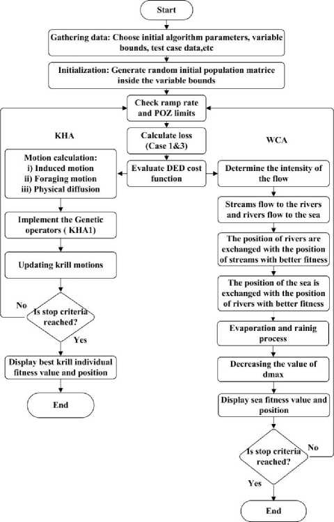
The flowcharts of the proposed methods are merged together and depicted in Fig.1.

×( ^River

-

^Stream )

^River ^{=      +} rand ^× C ×( ^Sea

^- X River )  (23)

Where rand is a uniformly distributed random number between 0 and 1. If any streams solution value is better than its connecting river, their position is changed (the stream becomes river and the corresponding river is considered as a stream). Also the position of sea and a river is changed if the river has a better solution than the sea.

The evaporation process has an important role in the algorithm preventing from getting trapped in local optima and rapid convergence. The concept of this process is taken from the evaporation of water from sea while plants transpire water during photosynthesis. Then clouds are formed from the evaporated water and release them back to the earth in the form of rain and make new streams and rivers flowing to the sea. When the distance between the river and sea is less than a small number named ^max the river has joined the sea and the evaporation process is applied, then the raining process will happen. ^max controls the search depth, near the sea. When a large value of ^max is selected, the search intensity is being reduced but its small value encourages it. The value of ^max decreases linearly at the end of each iteration.

The raining process is similar to the mutation operator in GA. The new randomly generated raindrops form new streams in different locations. Again the raindrop with the best function value among other new raindrops is considered as a river flowing to the sea. The rest of them are considered as new streams which flow to the river or go directly to the sea. For the streams that directly flow to the sea a specific equation which increases the exploration near sea is used, resulting improvements in the convergence rate and computational performance of the algorithm for constrained problems.

Start

Is stop criterk reached?

Is stop criteria' reached? /

Yes

End

KHA

WCA

Updating krill motions

Yes

Implement the Genetic operators ( KHA1)

Motion calculation: i) Induced motion ii) Foraging motion iii) Physical diffusion

Check ramp rate and POZ limits

Evaluate DED cost function

Initialization: Generate random initial population matrice inside the variable bounds

Gathering data: Choose initial algorithm parameters, variable bounds, test case data,etc

Determine the intensity of the flow '                        *                        :

Streams flow to the rivers and rivers flow to the sea

The position of rivers arc exchanged with the position of streams w ith better fitness

The position of the sea is exchanged with the position of rivers with better fitness

Evaporation and rainig process

Decreasing the value of dmax

Display sea fitness value and position

Г"

[ Display best krill individual fitness value and position

Fig 1. Flowchart of the proposed methods

IV. Case studies

In this paper, two different case studies are considered to show the feasibility of the proposed methods. The first system is A 5 unit system with valve point loading effect considering transmission loss and prohibited zones. In the second case study a 10 unit system with valve point effect but neglecting transmission loss is considered as a bigger and more complicated test case. All tests and scripts are written in MATLAB software on a Pentium IV dual core pc with 2 GB of RAM. Results and convergence characteristics are given in the remaining of this section.

• A.    5 Unit system

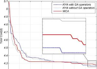
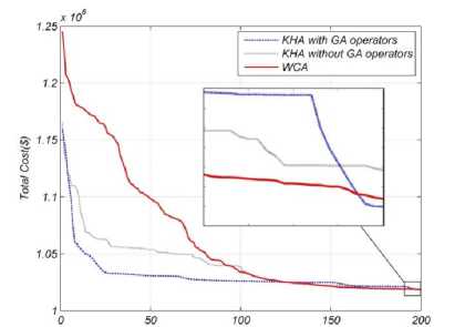
The first case study consists of valve point loading effect, transmission loss and prohibited zones of generators with the data and 24h load demand taken from [2] . The optimal algorithm parameters for KHA1 and KHA2 are Np_Op =150, Ct =0.5, 0)_n = =0.9, gbest = 0.02, _abest = 0.01 and for WCA are ⁼ 200, NS_r =40, ^max =0.1, c =2, и =0.1 . Table 1 shows the 24 hour dispatch of the units for KHA1. Table 2 also gives the minimum, average and maximum costs of three proposed methods in comparison with some other previously applied methods on this case study. The convergence characteristics of three methods are depicted in Fig.2 The distribution of objective function for 100 trials are given in Fig.3 and Fig.4 for KHA1 and WCA methods, respectively.

As it is given in the table, KHA1 had the best result between 3 methods with minimum cost of 42664.7744. WCA was close to KHA1 with the total cost of 42777.8503. In multiple runs, WCA had better mean cost with the average of 43118.8376 in 100 runs. KHA2 had good results but not good enough in comparison with two other methods.

• B.    10 unit system

4.2* --------------i-----------------------------1--------------i-----------------------------1--------------1--------------

The second case study is bigger than the previous one while only consists of valve point effects and the transmission loss is neglected. The system data for this case study is adapted from [10] . The optimal parameters for KHA1 and 2 are Np_Op = 180, Ct = 0.5, ^n = = 0.9 , gbest = 0.02, _abest = 0.01 and for WCA are Np_Op =220, NS_r =50, ^max =0.1, c =2, и =0.1 . Table 3 compares the results of the proposed methods with other methods in literature.

Table 1. 24h Dispatch of Units for Case 1 for KHA1

Hour	P1(MW)	P2(MW)	P3(MW)	P4(MW)	P5(MW)	Loss(MW)
1	15.398	72.812	60	119.266	146.148	3.4946
2	16.325	75.214	70	126.465	151.046	3.8777
3	17.686	90	77.24	136.789	158.127	4.6390
4	21.117	80	99.832	160	175	5.8504
5	23.212	93.105	113.251	160	175	6.5942
6	23.557	93.951	116.063	182.281	200	7.8198
7	25	98.526	140	195.735	175	8.3686
8	25	99.377	140	198.454	200.202	9.0903
9	25	104.935	143.87	214.833	211.464	10.0853
10	30	106.042	146.676	218.11	213.671	10.5444
11	30	107.969	151.58	223.837	210.236	11.0228
12	30	110.38	157.715	231.001	200.202	11.7122
13	30	106.042	146.676	218.11	200	10.5477
14	30	104.357	142.389	213.101	175	10.1798
15	25	99.377	140	198.454	175	9.2613
16	17.223	90	100	180	200.202	7.1994
17	20.923	90	98.737	180	214.899	6.6853
18	25	97.705	125	193.126	207.554	7.8796
19	25	99.377	140	198.454	200	9.1284
20	25	106.621	148.158	219.842	214.89	10.5554
21	30	103.038	140	209.195	207.554	9.8881
22	23.383	93.503	114.934	180.956	200	7.8535
23	20.262	90	94.214	156.724	171.717	6.1684
24	18.07	90	60	139.548	160.065	4.9872

Table 2. Results Comparison for Case 1

Method Production cost ($) CPU time (min) Min. value Mean value Max. value SA[2] 47356.0000 - - 5.86 GA[3] 44,862.42 44,921.76 45,893.95 3.3242 PSO[3] 44,253.24 45,657.06 46,402.52 3.5506 APSO[4] 44678 - - - ABC[3] 44,045.83 44,064.73 44,218.64 3.2901 MLS[5] 49216.81 - - 0.024 IPS[6] 46530 - - 4.53 KHA1 42664.7744 43426.0415 45023.885 3.021 KHA2 43071.6547 45345.0234 47839.7625 2.997 WCA 42777.8503 43118.8376 44204.7961 4.122 х 104

0      20     40     60     80     100    120    140    160

Iteration

Fig. 2. Convergence characteristic curve for case-1.

Table 4 also shows the generation data for 24 hours resulted from KHA1. Figure 5, 6 and 7 demonstrate the convergence curve for this case study and the distribution of the objective function for 100 trial runs for KHA1 and WCA,respectively.

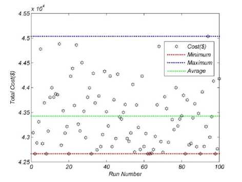
Fig. 3. Distribution of the objective function for 100 trial runs for 5-unit test system Using KHA1 (case 1)

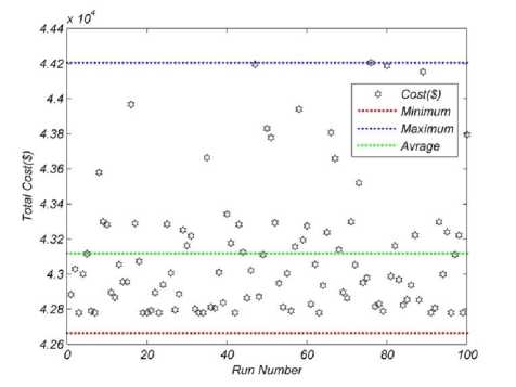
Fig. 4. Distribution of the objective function for 100 trial runs for 5-unit test system Using WCA (case 1)

Again the best result has been achieved using KHA1 with the minimum cost of 1,018557.2407 and WCA with total cost of 1018622.2205 was the second best method. Both methods had much better results than many other previously applied ones. The average cost for 100 runs for WCA was better than KHA methods with the mean cost of 1019394.0194.

• V.    Discussion

The execution time comparison between the methods shows that KHA had faster runs than WCA. That’s because in WCA, the raining process happens when the streams reach to the river. The scripts written for this process in economic dispatch problem must calculate the euclidean distance between two N dimensional vectors, which N is the number of generation units.

Iteration

Fig. 5. Convergence characteristic curve for case-2

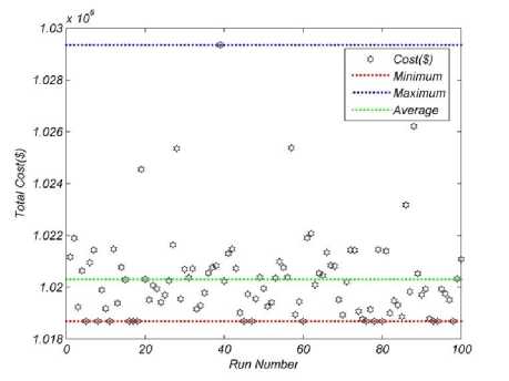
Fig. 6. Distribution of the objective function for 100 trial runs for 10-unit test system Using KHA1 (case 2)

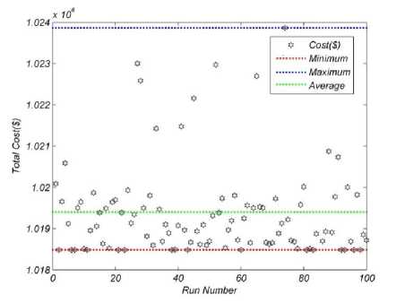
Fig. 7. Distribution of the objective function for 100 trial runs for 10-unit test system Using WCA (case 2)

This process takes time on bigger units. As it can be CPU times is bigger compared to the 5unit system. seen form table 4 the difference between WCA and KHA,

Table 3. Results Comparison for Case 2

Method	Production cost ($)			CPU time (min)
	Minimum value	Mean value	Maximum value
BCO-SQP [7]	1,032,200.000	-	-	3.24
ECE [8]	1,022,271.5793	1,023,334.9297	-	0.5271
AIS [9]	1,021,980.000	1,023,156.000	1,024,973.00	19.01
AHDE [1]	1,020,082.000	1,022,474.000	-	1.10
DE [10]	1,019,786.000	-	-	11.15
CDE3 [11]	1,019,123.000	1,020,870.000	1,023,115.00	0.32
KHA1	1,018557.2407	1020298.9975	1029345.2345	3.623
WCA	1018622.2205	1019394.0194	1023882.1018	7.3023
KHA2	1019420.8208	1023847.3745	131453.8725	3.0112

Table 4. 24h Dispatch of Units for Case 2 for KHA1

Hour	P1(MW)	P2(MW)	P3(MW)	P4(MW)	P5(MW)	P6(MW)	P7(MW)	P8(MW)	P9(MW)	P10(MW)
1	150.0150	135.0000	192.1056	60.0000	122.9001	124.3728	129.6065	47.0000	20.0000	55.0000
2	226.6120	135.0000	190.7530	60.0978	122.9175	122.9761	129.6282	47.0154	20.0000	55.0000
3	303.1590	215.0000	182.9477	60.0000	122.8698	122.4487	129.5718	47.0000	20.0029	55.0000
4	379.9372	222.2811	194.9529	60.9784	172.7400	123.4555	129.6208	47.034	20.0000	55.0000
5	456.4919	222.2770	191.5980	60.6096	172.7047	124.7049	129.6051	47.0000	20.0089	55.0000
6	456.5647	302.2770	209.4989	60.7132	222.6194	124.7292	129.5901	47.0000	20.0075	55.0000
7	456.5002	309.4742	279.3874	60.0000	222.6079	122.4415	129.5888	47.0000	20.0000	55.0000
8	456.4908	309.5506	301.8692	110.0000	222.6115	123.8669	129.6109	47.0000	20.0000	55.0000
9	456.4751	389.5506	323.2665	120.4737	222.6368	160.0000	129.5919	47.0054	49.9941	55.0000
10	456.4702	460.0000	320.8882	170.4737	222.5811	160.0000	129.5884	47.0044	52.0625	55.0000
11	456.8587	460.0000	340.0000	220.4737	224.9827	160.0000	129.6224	47.0000	52.0625	55.0000
12	456.4948	460.0000	339.6306	267.6389	222.5962	159.9882	129.6040	76.9988	52.0357	55.0000
13	456.4955	396.8704	307.7255	241.3151	222.6984	124.9052	129.6372	85.3169	22.0357	55.0000
14	456.5268	396.7835	292.2817	191.3151	172.7014	122.4642	129.5797	85.3120	20.0000	55.0000
15	379.8493	396.7478	295.7526	168.4366	122.8689	122.4607	129.5895	85.2945	20.0000	55.0000
16	303.2658	316.7478	302.0062	120.4340	73.0000	148.6514	129.5959	85.2990	20.0270	55.0000
17	226.6673	396.7478	299.8748	70.4945	73.0508	123.2250	129.5896	85.3233	20.0000	55.0000
18	303.2466	396.7913	297.3890	95.4079	122.8190	122.4268	129.5822	85.3373	20.0000	55.0000
19	379.8830	396.7952	295.2565	119.0312	172.7362	122.4457	129.5792	85.2730	20.0000	55.0000
20	456.4886	460.0000	313.9311	169.0234	222.6147	159.9978	129.6169	85.3274	20.0000	55.0000
21	456.5388	396.7995	311.5649	121.2520	222.6192	125.2692	129.6277	85.3288	20.0000	55.0000
22	379.7562	316.7995	275.2577	71.2520	172.7178	122.3637	129.5414	85.3118	20.0000	55.0000
23	303.2398	236.7995	196.5695	60.0000	122.8791	122.5971	129.6063	85.3089	20.0000	55.0000
24	226.6251	222.4868	186.1449	60.2484	73.0705	125.5110	129.6221	85.2913	20.0000	55.0000

• VI.    Conclusion

In this paper two novel heuristic algorithms have been applied on dynamic economic load dispatch problem. The first one, inspired from the movement of Antarctic krills, have been set as two sub-methods named KHA1 and KHA2 which differ in using and neglecting genetic operators. The second method named WCA, has been inspired from the cycling of water in the nature. The proposed methods have been applied on two common 5 and 10 unit DED case studies considering various DED constraints. Results, convergence characteristics and the distributions of DED objective function for 100 trial and runs for each methods show that WCA has more robustness giving great average results in multiple runs, while KHA1 gives unique best costs between multiple runs. Anyway both methods are totally new and powerful which can be applied on more complicated economic dispatch studies and also other optimization problems in power engineering studies.