Application of Texture Characteristics for Urban Feature Extraction from Optical Satellite Images

Published Online December 2014 in MECS

The enormous boost in the volume of remote sensing data available worldwide has necessitated the requirement of the development of feature extraction techniques for the extraction of geo-spatial features, with minimal human intervention. Automated feature extraction is the identification of geographic features and their outlines in remote-sensing imagery through postprocessing techniques that detects the features of interest [1]. Image interpretation, identification and characterization are vital and extremely challenging problems with abundant practical applications.

The subject of urban feature extraction from satellite images has always been an appealing topic of research among scientists and a lot has already been attempted in this field. Vincent Arvis et.al has worked on cooccurrence matrices extended for multispectral bands [2] and has reported promising results. Another study [3] by Örsan Aytekın and Arzu Erener proposes an algorithm for automatic extraction of both buildings and roads from complex urban environments using high-resolution satellite images, as this improves the overall performance of feature extraction. A detailed study on various Haralick features and an optimal feature selection algorithm is well described in [4].A combination of spatial metrics and texture measurements were examined for land-use categorization in [5] and has been implemented to Ikonos data using “object-oriented" approach. A texture based object recognition algorithm, in which a combination of gray-level co-occurrence matrix, Daubechies filters and rotated wavelet filters are used to get a high quality feature set, is proposed in [6].

Identification of urban objects like buildings from high-resolution satellite data has mainly focused on the spectral properties of the object being identified. Texture is an important characteristic used in recognizing the regions of interest in an image. Grey Level Cooccurrence Matrices (GLCM) is one of the earliest methods for texture feature extraction proposed by Haralick et.al. [7].Various statistical features like energy, entropy, homogeneity, mean, variance [8] etc which are extracted from the GLCMs, specifies the domain characteristics, which in turn helps to detect the regions of interest. Computation of all the features, results in a n-dimensional feature vector, which is highly cumbersome to handle. The assessment and optimization of these statistical parameters computed from textural features to discriminate regions of interest from their background class, is based on Jeffries-Matusita distance (JM-distance).The main advantage of Principal Components Analysis (PCA) is that it can reduce the number of dimensions, without much loss of information. This property is made use of in dimensionality reduction of the n-dimensional feature vector, so that the significant features can be identified for further processing. Reducing the dimensionality of feature vectors by combining the results of Jeffries-Matusita distance (JM-distance) and PCA has lead to an enhancement in accuracy and decrease in complexity and hence saving of computational time. The significant features are computed for the entire image and compared vis-a-vis the reference values for the region of interest and feature of interest is segregated. As an additional measure to ensure the detection of the desired feature and to avoid false detection, soil adjusted vegetation index, normalised difference vegetation index and normalised difference water index are assessed for reducing commission errors. The accuracy assessment, based on quantitative evaluation of true and false positives and negatives was also carried out as a final step.

The succeeding section presents the developed algorithm based on Gray Level Co-occurrence matrices, the selection of various statistical textural features, various criteria for dimensionality reduction, segregating region of interest and the background pixels based on selected texture feature values and soil index along with a brief theoretical background of the same. The third section discusses the data set used, which comprises of a high resolution satellite image, which images the city of Hyderabad to map varying ground terrains and the results obtained. The subsequent section deals with the evaluation of the feature extraction algorithm by assessing the omission and commission error percentage.

• II.    METHODOLOGY

This section gives in detail the proposed algorithm, which initially evaluates the Gray Level Co-occurrence matrix for a predefined number of samples, compute the texture features for all samples, identify the optimal features and finally assess the corresponding values for the test image, so as to classify the relevant feature in the candidate image. The detailed flow is presented in figure 1.

• A. Gray Level Co-occurrence Matrix

The Gray Level Coocurrence Matrix (GLCM) method is applied for extracting second order statistical texture features any element of the matrix P (i, j | ∆x, ∆y) is defined as the relative frequency with which two pixels, separated by a pixel distance (∆x, ∆y), appear in a given neighborhood, one with intensity i and the other with intensity, j[9]. The interrelationships between the grey values in an image are transformed into the co-occurrence matrix by kernel masks such as 3*3, 5*5, 7*7 and so on. During the transformation into the co-occurrence matrix space from the image space, the neighboring pixels are considered in one or the other of the four defined directions such as 0°, 45°, 90°, and 135° along with displacements 1,2,3,4 and 5 in these axes. To summarize, GLCM texture measure depends upon kernel mask size or window size and the directionality. Many textural features such as Energy, Homogeneity, Contrast, Correlation, Entropy, Dissimilarity, Mean, Variance and Sum of Squares are generated from these GLCMs. While contrast assesses the local variation in the gray level, correlation provides the joint probability of occurrence of pixel pairs and energy gives the sum of squared pixel values of GLCM. Homogeneity refers to the closeness of distribution of elements to the diagonal. Hence, a proper selection of GLCM computational parameters will help in proper utilization of the generated GLCMs for calculating textural features from them, for further processing.

• A.1 Selection of Optimal value for Displacement,d

Displacement values can vary in the range of values like 1, 2 3 4...10. The application of relatively high displacement values to a fine texture might yield a GLCM that fails to capture detailed textural information [10]. This is justified, as a pixel has more correlation to other closely located pixel than the one located far away.

A reasonable selection of displacement values in the range 1,2,3,4 and 5 was applied for the computation of GLCMs, so that the overall classification accuracy can be met.

• A.2 Selection of Optimal value for Orientation angle,

There can be eight orientations and hence eight choices for α, which are 0°, 45°, 90°, 135°, 180°, 225°, 270° or 315°. As per the definition of GLCM, the co-occurring pairs obtained by choosing θ equal to 0° and 180° will be similar. In this context, only four values of α need be considered for the computation of GLCMs.

This approach hence focuses on angular offsets of 0°, 45°, 90° and 135° for the generation of GLCMs.

• A.3 Selection of Optimal value for window size

Selection of the size of the moving window is a critical parameter, since various class types has to be extracted over a local area of unknown size and shape.

The textural information has to be extracted over as large an area as possible. In some cases, the window selected may cover more than one texture class [11]. This highlights the need for a trade-off between various window sizes that give invariant texture measures and sufficient ratio of between-class variance.

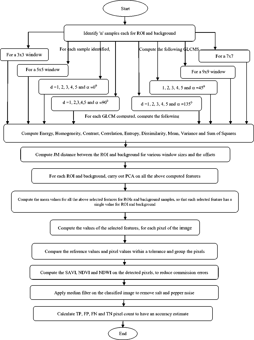
Fig 1. Flow Chart of the proposed algorithm

This study has been conducted with varying window sizes as 3x3, 5x5, 7x7 and 9x9, so as to ensure that the generated GLCMs provide sufficiently accurate texture features for precise classification.

A.4 Generation of GLCMs with different parameters

As discussed in the previous sections, the window size, the displacement and the orientation angle play a key role in the generation of GLCMs. This algorithm proposes to compute 1 GLCM each for

• • Each window size ie. 3x3, 5x5, 7x7 and 9x9.Hence,

• 4 GLCMs are computed from the four kernel masks.

• • Each displacement ie.1,2,3,4 and 5 with each orientation angle, 0°, 45°, 90°, 135°.Hence, 20

GLCMs are calculated from the combination of displacements and orientation angles.

Thus, a total of 24 GLCMs are computed for each of the sample identified. The algorithm then proceeds to compute the texture parameters from these GLCMs.

A.5 Estimation of Texture Parameters

The preliminary step in image classification is the estimation of various texture parameters viz. Energy, Homogeneity, Contrast, Correlation, Entropy, Dissimilarity, Mean, Variance and Sum of squares.

The following equations are used to compute the above mentioned parameters. G is the number of gray levels used, ц is the mean value of P and ц_х, ц _у, п _х and a _y are the mean and standard deviations of P_x and P_y . P_x(i) is the ith entry in the matrix obtained by summing the rows of P(i,j)[9]

G-l

Px(i)=Zj=0 P(i.D(1)

G-l

Py(j)=Z,=0 P(I-D(2)

G-l G-lG-l

Цх = Z,=0 i Zj=0 P(i. j) = Z i=0 i Px(i)(3)

G-l G-lG-l

Цу = Zt=0 jZ J=0 P(i,j) = Zj=0 j Py(j)(4)

G-l          G-lG-l a2 = Z(=0 (i —  Цх)2 Zj=0 P( i. j) =Z(=0 (Px (О-Цхб))2

G-l          G-lG-l ay2 = Zj=0 0-  Цу)2 Zi=0 P(U ) =Z J=0 (Pу (j) - Цу (j))2

And the corresponding texture feature parameters are generated as

Angular Second Moment or Energy = Z Z P (i.7)2

i j

G-l       G G

Contrast = z n2 {^=г Z=г P(i.;)} , |i-j|=n(8)

n=0

G-l G-l

Homogeneity =Z Z   ^ P(i,j), x=(i-j)(9)

i=0;=0

G=1G=1

Entropy =Z Z    P(i.j') x log ((P(i,j))(10)

i=07=0

Correlation= ZiZi{(iJ)p(U) ~ ^^(11)

G-l G-l

Sum of Squares, Variance = Z Z     (i- м) 2 Р(Ц)

i=07=0

2G-2

Mean = Z    iP x+y(i)(13)

i=0

G-l G-l

Dissimilarity = Z Z    P (i. j )|i-7!(14)

i=07=0

The above mentioned texture features are computed from all the 24 GLCMs that are created using the various combination of window size, displacement and orientation angle as mentioned in the previous subsection.

Since 8 texture feature measures are to be assessed for every GLCM, this will result in 192 texture measure values for every sample, which acts as a pointer in image classification.

• B. Statistical Separability Analysis for Feature Selection

Any feature can be identified using this proposed algorithm. In this paper, we focus on the identification and extraction of buildings. Separablity tests are necessary to assess the potential of the selected feature measures in image classification. These help in providing information about the discriminative ability of a parameter in detecting between two discrete classes and the efficiency of the selected training data in image classification.

The J-M distance [12] is a function of separablity that evaluates both class mean and the distribution of the values about those means and works on n-number of bands. This estimates how good a resultant classification will be. The JM distance between two class i and j, for a multivariate Gaussian distributions is given by:

Jij = √2(1-e^(-Bij)                 (15)

where B ij ,the Bhattacharya distance is,

_D 1 z        _AT Z^{Z + Z}7 X/           11 [^|(Zi + ^Z7 ⁾ 1 ² П

B ij = -(m i - m j ) (     ,.     ^ (m i - ^m k ⁾+ 2 1n[ _V |z_i| V|E j । ]

where m_i and m j are the class mean vectors and

∑ I and ∑ j   are the class covariances. J ij ranges from

0 to 2 with 2 indicating the highest separability.

The application of JM-distance is carried out in this design in the following way.

• •    Each texture feature viz. energy, correlation, contrast, dissimilarity etc. is computed for a single parameter viz. 1 value of window size or a single value of displacement at a fixed offset.

• •    Values are paired by grouping corresponding feature values for the region of interest and the background.

• •    As a final step, compute the JM distance for the paired values.

• •    The texture features which give the maximum JM distance provide the class with maximum separability.

Thus, it is possible to choose those combinations of computational parameters, which yields maximum separation and hence facilitate feature classification.

The above described steps are implemented and the texture feature values are grouped together with corresponding computational parameters. The subsequent step in this algorithm is the computation of JM distance for these paired textural features. An assessment of JM distance reveals that the following textural measures computed with the below referred parameters has resulted in the maximum JM distance and only need to be considered for further processing.

• •    Window size of 3x3

• •    Displacement of 1

• •    Orientation angle of 0⁰

For the following textural features

• •   Variance, Energy, Contrast and Homogeneity

• C.    Dimensionality Reduction Techniques

The calculation of the 8 texture measures for each GLCM will end up in a 24x8 feature vector, which is complicated to handle. A technique to resolve this problem is to use dimensionality reduction techniques. Principal Components Analysis and Linear Discriminant Analysis are the two most popular techniques used for dimensionality reduction. This paper discusses the use of PCA method for reducing the dimension of the feature vector.

C.1 Principal Component Analysis

The principal components of the distribution of features or the eigenvectors of the covariance matrix of the feature vectors, is sought by treating every feature as a vector in a very high dimensional vector space.PCA is applied on this feature vector space, which facilitates in finding a set of the most representative projection vectors so that the projected samples maintains a large amount of information about original samples. An advantage of PCA is that around 90% of the total variance is contained in less than 10% of the dimensions.

In this paper, PCA is carried out on a 24x8 feature vector space on every sample. It builds M eigenvectors for an N x M matrix ie, 8 eigen vectors are computed from the vector space. They are arranged from maximum to minimum, where the maximum eigenvalue is associated with the feature that finds the most variance, so that it can contribute significantly for image classification. Thus, PCA helps in dimensionality reduction from 8 to 3, where only 3 eigen vectors have significant eigen values, and hence only these features have a say in image classification. These eigen vectors correspond to energy, homogeneity and contrast and will only be used for further processing.

• D.    Evaluation of Reference Values for Textural Measures

The outcome of the execution of the preceding steps is a value corresponding to each texture measure for each region of interest/ background. To ensue further processing, a reference mean value is figured for every texture measure with each combination of computational parameters.

To explain further, a reference mean value is assessed for the texture measure, energy, computed using 2 combinations, ie. With a 3x3 window and another with a displacement 1 and an orientation angle of 0o .This is repeated for other texture measures viz. homogeneity, variance and contrast. Thus, reference values are obtained for all chosen texture measures with the combinations of computational parameters like window size, displacement and orientation angle for region of interest and background.

• E.    Segregation of Feature of Interest in Any Image

• E. 1 Analysis of Candidate Image

Having obtained the mean values for all the textural measures with the significant combinations of computational parameters, the next step is to classify the various pixels in the image.

A 3x3 window is identified around every pixel in the image. For every window, compute the noteworthy texture measures viz. energy, homogeneity, contrast, and variance. In addition to this, the texture measures are also evaluated with the specified displacement 1 with an orientation angle of 0o. To summarise, each pixel will have two sets of texture feature vector that are calculated based on the chosen computational parameters.

• E. 2 Comparison with Reference Values

The processing of the above step results in two sets of values for every pixel corresponding to each texture feature. Subsequently each pixel in the image is to be classified based on these texture values.

The texture measures computed for every pixel are compared with their corresponding reference counterparts with a marginal tolerance. Depending on the outcome of the comparison, the pixels are classified as feature or background.

• E.3 Reducing Commission Errors

The algorithm based on selection of significant texture feature measures and grouping of pixels based on their values will result in the exact classification of a major chunk of pixels. Equally important is the need to reduce commission errors, which will significantly affect the quality percentage. To avoid such a scenario, it becomes mandatory to check that every pixel that is detected as a feature is itself a feature in ground truth. The aim of this algorithm is to minimize the commission errors, ie, to minimize the number of background pixels inadvertently identified as feature.

E.3.1 Soil Adjusted Vegetation Index (SAVI).

The assessment of soil adjusted vegetative index is one of the best indices to This is computed as

SAVI = avoid over detection of features.

(NIR - RED)*( 1+L) (NIR+RED+L)

where NIR is the reflectance value of near infrared band, RED is reflectance of the red band and L is the soil brightness correction factor. The value of L varies by the amount of green vegetation, with very high vegetation regions having L=0 and L=1 in areas with no green vegetation. Generally, an L=0.5 works well in most situations and is the default value used. Hence lower the value, the lower the amount of green vegetation, which depicts more of soil characteristic and indirectly pointing to the fact that a higher value is indicative of the feature being detected.

E.3.2 Normalized Difference Vegetation Index (NDVI).

Another index that can contribute significantly in image classification is Normalized Difference Vegetation Index (NDVI). NDVI takes into account the amount of infrared reflected by plants. The NDVI ratio is calculated as

NDVI =

(NIR-RED )

(NIR+RED )

Values of NDVI in the range of less than 0.1 correspond to barren areas of rock, sand, snow, exposed rock or nil vegetation which can aid in isolating the vegetation areas and detecting the interested features.

E.3.3 Normalised Difference Water Index (NDWI)

Normalized Difference Water Index (NDWI) [14] has been defined as

NDWI = ^{(Gree n NIR)}

(                 )

This index maximizes the reflectance of water using green wavelengths and also takes into consideration the high reflectance of NIR by vegetation values for water features, while vegetation and soil have zero or negative values. Thus, low values of NDWI and soil features. Due to this fact, this index assumes positive help in segregating and isolating water features.

E.3.4 Algorithm Formulation by means of Indices

Evaluation of indices is used as an effective means to reduce the commission errors that might have crept into the detection of feature of interest, by employing texture measures.

The methodology comprises of an initial classification of pixels based on texture measures and further removing the false positive pixels by making use of indices. A combination of a high value of SAVI and low values of NDWI and NDVI can be applied to confirm the identity of detected pixels as those of feature of interest.

E.4 Application of Median Filter

The output image after the above filtering processes is passed through a median filter to remove the salt and pepper noise from the image. The median filter [15] is a simple rank selection filter that removes impulse noise by replacing the luminance value of the center pixel of the filtering window with the median of the luminance values of the pixels contained within the window.

• F. Estimation of Achieved Accuracy

Assessing and quantifying the achieved accuracy is an essential requisite for any feature extraction algorithm. To attain this objective, it is necessary to evaluate the number of true negative (TN), false positive (FP), false negative (FN) and true positive (TP) pixels. TP refers to the pixels detected as feature of interest, FP refers to the wrongly detected pixels as features, and FN refers to the regions, which could not be detected as feature of interest, although they exist in the ground truth. These quantities help us in evaluating the often cited terms such as

.             TP+TN Accuracy = J TN+FP+FN+TP	(20)
Precision =   PP FP+TP	(21)
True Positive Rate = TP FN+TP	(22)

• III.    Results and Discussions

• A.    Data Set

The data set selected for the validation of the developed algorithm is a fused image of Resourcesat-2 and Cartosat-2. The Resourcesat-2 sensor employed for this fused image generation was multispectral Liss-4 with a spatial resolution of 5m. The Cartosat-2 has a panchromatic camera with a spatial resolution of less than 1m.The merged image is a multispectral image with a spatial resolution of 1m.

• B.    Assessment of Texture Parameters based on JM-distance

As mentioned in the previous sections, the implementation of this algorithm starts with identifying a reasonable number of samples for the region of interest and the background. The number of training samples needs to be around 1% to 5% of the full image. For proper accuracy assessment, an adequate number of testing data samples is required for the selected feature of interest. In this case study, the selected feature of interest is buildings. For each of the identified samples; compute 24 GLCMs obtained from the five displacements for each value of orientation angle specified and selected window sizes. There are 8 texture parameters to be calculated for each GLCM, accounting the total count of texture measures to be assessed to 192 for each sample. Consequent to computing the texture measures, the next step is to carry out separability tests to assess the discriminative ability of selected parameters. This is achieved by computing the JM-distance for each of the combination of orientation angle, displacement and window sizes between background and region of interest. The following table gives the JM distance computed for various texture parameters.

Table 1. Maximum JM distances for different combinations

Maximum JM distances for various orientation angles computed for different displacements ,d=1,2,3,4 and 5
	0o	45o	90o	135o
Contrast	1.0769	0.53228	0.38067	0.62784
Energy	1.2307	0.61830	0.82315	0.46638
Homogeneity	1.3230	0.64504	0.91382	0.14066
Dissimilarity	0.5913	1.10773	0.66134	0.19363
Entropy	0.8529	0.62508	0.63638	0.52466
Variance	1.9999	1.99998	1.99997	1.99996
Mean	0.8350	0.79200	0.37820	0.43250
Correlation	0.9671	0.39964	0.36988	0.57787
Window sizes	3x3	5x5	7x7	9x9
	1.7772	1.75359	1.73018	1.70424

The JM distance acquires values from 0 to 2, where 2 indicated the maximum separability. An analysis of the above table shows that the JM distance has maximum values for variance, followed by homogeneity, energy and contrast and hence these parameters can be used for image classification.

Image classification based on texture measures require information regarding the orientation angle and displacement for which the maximum JM-distance is observed. From the results, it is observed that these values correspond to an orientation angle of 0o and displacement 1.Hence further steps in image classification will focus only on computing the above mentioned four texture measures being computed for 0o orientation angle and a displacement value of 1.

• C.    Assessment of Eigen Values for Dimensionality Reduction.

As a measure to achieve dimensionality reduction from 8 feature vectors, PCA is carried out. The features with high eigen values are found to contribute significantly for image classification. In this context, energy, homogeneity and contrast have significantly high eigen values compared to the others, which help in dimensionality reduction from 8 to 3

• D.    Image Analysis with reference to the key feature vector

The subsequent step is to evaluate a mean reference value for all the chosen feature vectors, which include energy, homogeneity, contrast and variance computed for a 3x3 window and an orientation angle of 0o with displacement, 1.This is carried out for pixels of both region of interest and background.

Consequent to the reference vector generation, the next step is to analyse the candidate image and classify the features. A 3x3 window is identified around each pixel and a GLCM is computed, for which the four identified key feature vectors are assessed. In addition to this, GLCMs are computed with an orientation angle of 0o with displacement,1 for each pixel. Thus, every pixel corresponds to eight feature values, two for each of the feature parameters viz. variance, energy, homogeneity and contrast. The individual values evaluated for each pixel are compared with the pre-defined reference value within a tolerance band (=0.5). The pixels which satisfy the laid down criteria are identified as the pixels corresponding to that of the feature of interest or that of the background.

• E.    Reduction of Commission Errors

The estimation of the reference texture measures and their comparison with individual pixels may not result in the avoidance of commission errors. To overcome this difficulty, indices are computed and are calculated as a cross-check measure. The SAVI, NDVI and NDWI values help us to rule out the presence of pixels other than that of the feature of interest, viz. water, barren soil and vegetation. The bench mark values for identifying the feature are selected as 0.06 for SAVI, 0.2 for NDWI and 0.02 for NDVI. The individual pixels are classified as feature of interest if its SAVI is greater, NDWI is lesser and NDWI is also lesser than their respective defined threshold values. This check helps to reduce the commission errors that have been introduced by the earlier detection process.

• F.    Median filter for Noise Removal

The output image after the classification is passed through a median filter to remove the salt and pepper noise, if any, present in the output image. This filter replaces the luminance value of the center pixel of the filtering window by the median of the luminance values of the pixels contained within the window. The median filters remove thin lines and random image details at low noise densities.

• G.    Quantification of Achieved Accuracy

The data set mentioned in Sec. 3.1 covers the city of Hyderabad. The data set covers land mass, water body, buildings, and green vegetation and opens areas. The test images (Fig. 2- Fig. 5) are selected portions of the data set, so as to have a wide coverage of the features. The algorithm performance is validated for varied types of regions to assess the efficiency of the algorithm in detecting the feature of interest, ie buildings. The test images in Fig. 2 and Fig. 3 are semi urban areas with greener pastures also, while Fig. 4 has a water body in the image. The algorithm is evaluated in Matlab environment. Accuracy assessment is performed by pixel-based evaluation on the basis of visual assessment of the features in the input image and the features identified by the algorithm. It can be seen that the percentage of omission and commission varies with the regions present in the candidate image.

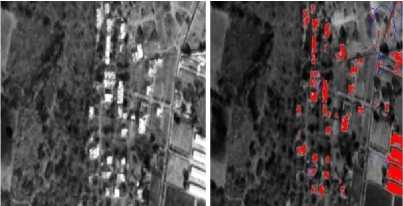
Fig. 2. Test image 1 and feature extracted image

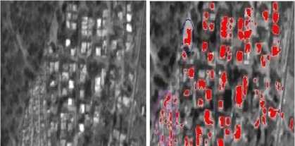
Fig. 3. Test image 2 and feature extracted image

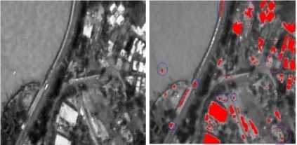
Fig. 4. Test image 3 and feature extracted image

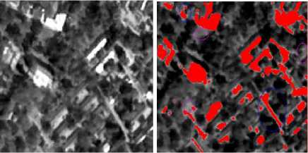
Fig. 5. Test image 4 and feature extracted image

The following table gives the accuracy, precision and true positive rates for the various test images

Table 2. Accuracy, Precision and TPR for the selected test images

	Accuracy (%)	Precision (%)	True Positive Rate (%)
Test image 1	98.51	84.92	86.70
Test image 2	98.02	92.69	84.10
Test image 3	97.23	77.66	81.66
Test image 4	98.29	88.12	87.41

It can be inferred from the above table that the accuracy and precision depends on the ground texture of the area under study. The least precision and accuracy is observed in test image 3, due to its higher percentage of barren land with less vegetation and false detection of barriers near the water body as buildings. A true urban environment gives very good results, in terms of both precision and accuracy, as can be seen from the results of test image 2.

• IV.    Conclusion

It can be very well observed that the proposed algorithm qualifies very well for identification and extraction of selected feature viz. buildings in high resolution satellite images. This method also evaluates the various indices to reduce the proportion of under/over detection. The overall performance of this algorithm has been found to be satisfactory as can be inferred from the results.

To improve the accuracy and precision in feature extraction and to ensure consistency, the authors plan to superimpose the edges of various features obtained by edge detection techniques on the extracted features. This will facilitate in reducing considerably the percentage of false detections. In addition, it is planned to incorporate region growing techniques as an additional measure to improve the accuracy of feature detection.