Applied Computational Engineering in Magnetic Resonance Imaging: A Tumor Case Study

Published Online June 2014 in MECS DOI: 10.5815/ijigsp.2014.07.01

Solving the equation E0 = EIN in f(0) yields the signal resilient to interpolation:

f 0 ) = F(E o ( x ) = Ein( x )) = F( x ) (6)

The signal resilient to interpolation is a function of the variable x, therefore changing in between the intra node coordinates. The signal resilient to interpolation can be calculated under the assumption that the model polynomial function fitted to the original signal benefits of the property of second-order differentiability in its interval of definition. The definition of the IntensityCurvature Functional is:

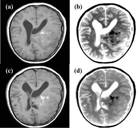
Fig 1: The tumor MRI is shown in (a) and in (c), the matrix size is 512×512 pixels with 0.49mm × 0.49mm as pixel size. In (b) and in (d) is shown the signal resilient to interpolation of the images seen in (a) and in (c) respectively, with a visible highlight on the region of the tumor with the affected area characterized by the dark regions most likely showing fluids like blood and water. The images were cropped so to show the regions of interest.

AE(x) =

Jo(xL ^e in ^{( x )}

One is that the distinction between gray and white matter of the brain is more visible in the signal resilient to interpolation images in (b) and in (d); and the other one is that the observation of (a) versus (b) and of (c) versus (d) demonstrates higher level of details in the signal resilient to interpolation images which would not be otherwise observable in the original MRI. The aforementioned

observation is more evident when looking at the images in (a) and in (b) of Fig. 1.

Fig. 2 serves the purpose to illustrate that, with brightness-contrast enhancement set to a particular level, it is possible for the signal resilient to interpolation images (see Fig. 2b and Fig. 2d) to display in negative, the same level of details of the original MRI. The contour line of the tumor is well discernible in (a) and in (b) along with the details relevant to the fluids shown in bright and dark in the two images. It is interesting to note the slight difference between the image in Fig. 2a and the image in Fig. 2b, specifically the tumor structure seen in (a) is missing at the location indicated by the dark arrow in (b). In both of the images seen in (c) and in (d) the region of the tumor is well demarcated showing the affection of the

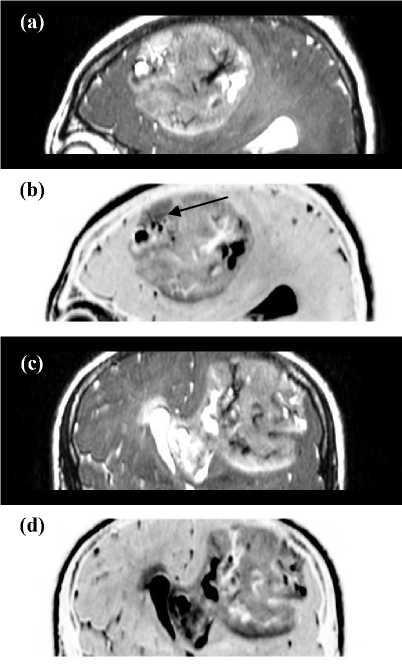
Fig 2: The tumor MRI is shown in (a) and in (c), whereas the signal resilient to interpolation is shown in (b) and in (d). The matrix size is 512×512 pixels with 0.39mm × 0.39mm as pixel size. Likewise in Fig.

1, data in (a) and in (c) are fitted with the bivariate cubic Lagrange model function and re-sampled with (x, y) = (0.01mm, 0.01mm). The signal resilient to interpolation highlights on the region of the tumor with specific focus on the fluids which are shown in dark and in bright in the images. In this figure though the signal resilient to interpolation acts as a negative of the original MRI, and the level of details of the signal resilient to interpolation is not superior to the MRI of (a) and (c). The images were cropped so to focus on the regions of interest.

Ventricles because of the presence and the extension of the tumor. In summary, Fig. 2 is a case in which is objective to report that the signal resilient to interpolation offers complementary information but not additional information in reference to the original MRI.

Fig. 3 shows a typical case of complementariness between the signal resilient to interpolation and the MRI. The brightness-contrast enhancement has been set to values making a comparison which is on the same basis of objectiveness. While looking at the MRI of Fig. 3a and Fig. 3c the following observations can be made. The extension of the tumor, the pressure exercised by the tumor onto the ventricles, the fluids which are presumably water and/or blood, and the nuances of the region of the tumor. Within the context of complementariness, the signal resilient to interpolation shown in Fig. 3b and in Fig. 3d confirms the anomaly seen in MRI. Specifically, when looking at the regions inside the white circles in Fig. 3 it is possible to have confirmation of the extension of the tumor in reference to the tumor contour line (see bottom part of the image located inside the circles).

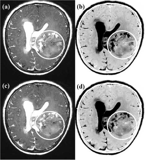
Fig 3: The MRI with the tumor is shown in (a) and in (c), the signal resilient to interpolation is shown in (b) and in (d). The complementary information provided by the signal resilient to interpolation focuses on the bright and dark regions of the tumor seen inside the circles, most likely fluids like blood and/or water. The level of details seen in (b) and in (d) is similar to the original MRI. The matrix size is 512×512 pixels with 0.39mm × 0.39mm as pixel size. The images were cropped so to focus on the regions of interest. The model polynomial function fitted to the images shown in (a) and in (c) is the bivariate cubic Lagrange and the intra-pixel re-sampling coordinate is (x, y) = (0.01mm, 0.01mm).

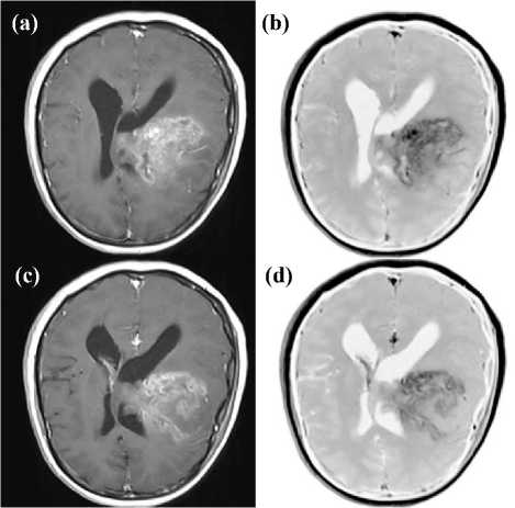
Fig 4: The original MRI is shown in (a) and in (c) and the signal resilient to interpolation is shown in (c) and in (d). The level of details of the tumor region is equally visible in the signal resilient to interpolation images in (b) and in (d) when compared to the MRI in (a) and in (c). The dark region is presumably blood and/or water. The matrix size of the images is 512×512 with pixel size of 0.49mm × 0.49mm. The images in (a) and (c) were fitted with the bivariate cubic Lagrange polynomial and they were re-sampled of the misplacement (x, y) = (0.01mm, 0.01mm).

An interesting observation visible in Fig. 3 is that the Cerebrospinal Fluid (CSF) is imaged with the same color (in dark color) of the fluids of the tumor (see (a) and (c)), and as far as regards this, the opposite is visible (in bright color) in the images of the signal resilient to interpolation in Fig. 3b and in Fig. 3d.

The dark nuances seen in Fig. 4 demonstrate, as far as regards the signal resilient to interpolation images seen in (b) and in (d), that the level of details of the tumor is quite similar to the MRI image seen in (a) and in (c) respectively. The images in Fig. 4 have been adjusted to the level of brightness-contrast enhancement so to make an objective comparison. The tendency seen in Fig. 2, Fig. 3 and Fig. 4 is though, that one of complementariness of the signal resilient to interpolation to the MRI, whereas in Fig. 1 the tendency of the signal resilient to interpolation is that one of offering additional information about the tumor to the MRI.

• B.    The Intensity Curvature Functional

Fig. 5 shows the combined use of the signal resilient to interpolation and the Intensity-Curvature Functional. The signal resilient to interpolation was calculated when fitting the parametric bivariate quadratic B-Spline model function [21-23] (see (c) and (d)) to the original MRI shown in (a) and in (b), whereas the Intensity-Curvature Functional (see (e) and (f)) was calculated when fitting the bivariate linear model function. The misplacement used to re-sample the images so to obtain Fig. 5c and Fig. 5d is (x, y) = (0.9mm, 0.9mm), with the value of the parametric constant set to 2.54, and the misplacement used to re-sample the images so to obtain the images seen in Fig. 5e and in Fig. 5f is (x, y) = (0.01mm, 0.01mm).

Fig. 6 shows the Intensity-Curvature Functional calculated on the basis of the original MRI seen in Fig. 1a and Fig. 1c. As anticipated earlier the main characteristic of the Intensity-Curvature Functional is that one of displaying the third dimension perpendicular to the image plane.

The third dimension reveals information about the anatomical structures of the human brain and as such also the tumor structures are highlighted. In this section of the paper, the Intensity-Curvature Functional was calculated when fitting to the MRI the bivariate linear model function and the intra-pixel re-sampling coordinate is: (x, y) = (0.5mm, 0.5mm). An important characteristic shown in Fig. 7 is the highlight of the fluids of the tumor.

When looking at Fig. 7 in comparison to Fig. 2a and Fig. 2b, it is possible to recognize that what was seen in the aforementioned pictures in bright and dark is here reproduced with an elevation from the imaging plane and such elevation adds information to the original MRI as far as regards the anatomy of the tumor structures. In general, it is visible from the pictures reported in this section that the most important capability of the Intensity-Curvature Functional is that one of presenting information which is not observable in the original MRI and such information pertains to the third dimension given by the IntensityCurvature Functional to the anatomical structures of the brain and more specifically to the anatomy and the details of the tumor.

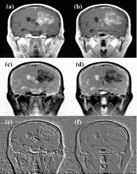
Fig 5: The original MRI is shown in (a) and in (b). The signal resilient to interpolation is located in the images shown in (c) and in (d). The Intensity-Curvature Functional is shown in (e) and in (f). The matrix size of the images is 512×512 with pixel size of 0.45mm × 0.45mm. While the signal resilient to interpolation clearly shows complementary information to the original MRI, the Intensity-Curvature Functional adds information to the original MRI when showing the depths of the anatomical structures of the tumor. The depths are more visible in (e) than in (f). The images were cropped so to highlight the regions of interest.

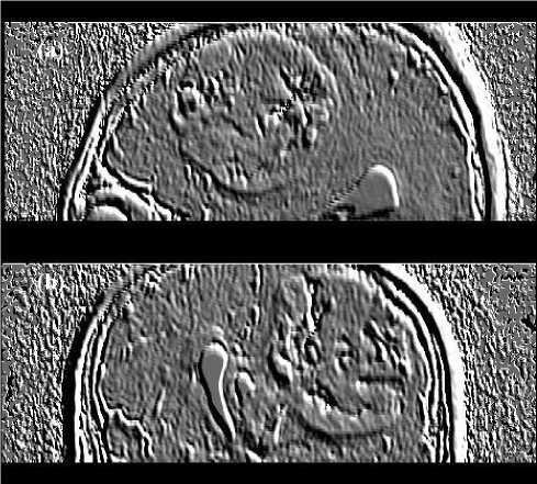
Fig 7: The Intensity-Curvature Functional of the MRI shown in Fig. 2a is on display in (a), whereas the Intensity-Curvature Functional of the MRI shown in Fig. 2c is shown in (b). The characteristics of the images in (a) and in (b) is that of presenting the third dimension of the tumor structures, along with the CSF (see (b)), which appears elevated along the axis perpendicular to the imaging plane.

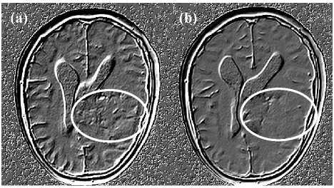
Fig 6: The Intensity-Curvature Functional of the MRI seen in Fig. 1a is shown in (a), whereas the Intensity-Curvature Functional of the MRI seen in Fig. 1c is shown in (b). The elevation of the cortex with respect to the cerebrospinal fluid (CSF) is visible from the pictures and also the contour line of the ventricles appears as such to give the perception of the third dimension perpendicular to the image plane. The tumor structures are highlighted in the regions inside the white ellipses (see

Fig. 1a and Fig. 1c for reference).

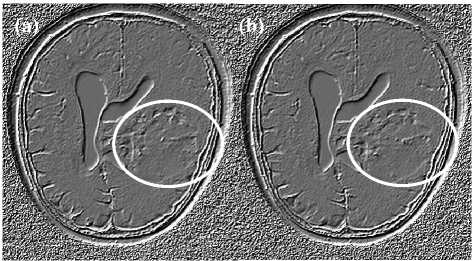
Fig 8: The Intensity-Curvature Functional of Fig. 3a is shown in (a) and the Intensity-Curvature Functional of Fig. 3c is shown in (b). These pictures present another evidence of the capability of the IntensityCurvature Functional to build the third dimension perpendicular to the image plane. In the specifics, the ventricles and the CSF are shown with an elevation when compared to the cortex and more specifically when compared with the anatomy of the tumor (see regions inside the white ellipses).

Clearly, Fig. 7 shows that the Intensity-Curvature Functional is capable to identify the tumor contour line. In Fig. 8 the accent is on the ventricles, the CSF and the anatomical structures of the tumor. The pressure exercised by the tumor on the ventricles and the third dimension of the tumor structures are visible. Specifically, what was seen in white (most presumably fluids) in Fig. 3a and in Fig. 3c is here seen in Fig. 8a and in Fig. 8b with an elevation from the image plane. It is worth mentioning that the combined information provided through the signal resilient to interpolation images seen in Fig. 3b and in Fig. 3d, which is complementary to the original MRI, is now corroborated with the additional information provided through the Intensity-Curvature Functional shown in Fig. 8a (calculated from Fig. 3a) and the Intensity-Curvature Functional shown in Fig. 8b (calculated from Fig. 3c).

The additional information provided through the Intensity-Curvature Functional images shown in Fig. 9 is relevant to the white nuances seen in Fig. 4a and Fig. 4c. The Intensity-Curvature Functional in the case presented in Fig. 9 is able to build a third dimension on the basis of what in Fig. 4 are shown as fluids of the tumor. This is not the first instance as it was seen in the previous figures seen in this section, which show that the fluids can have a third dimension extracted by the Intensity-Curvature Functional.

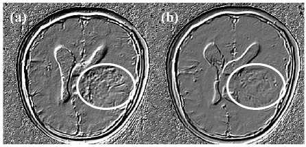
Fig 9: The Intensity-Curvature Functional of the MRI shown in Fig. 4a is shown in (a), and the Intensity-Curvature Functional of the MRI shown in Fig. 4c is shown in (b). A remarkable feature of the IntensityCurvature Functional images is the making of the third dimension of the white nuances seen in Fig. 4 (see regions of the tumor inside the white ellipses). Also, the contour line of the ventricles is elevated from the inner CSF and the cortical region appears at the same elevation of the ventricles (see the contour white line).

• IV.    Discussion

The major findings of the research herein presented are congruent with the following concept. An image processing algorithm which is intended to perform feature extraction from the original image cannot extract any realities from the original image which do not exists in the image. Think of the previously stated concept likewise filter theory. A filter applied to a signal can extract frequencies located in the signal but cannot make frequencies out of the signal that are not located in the signal. The congruency of the aforementioned logic is in harmony with the results seen from the calculation of the signal resilient to interpolation from the original MRI. We have seen through the results presented in this paper that the tendency of the signal resilient to interpolation is to reproduce the MRI with similar, if not equal, level of details. However the reproduction of the details of the signal resilient to interpolation happens in a domain which is not the same as the one of the MRI, and thus it was seen that the signal resilient to interpolation adds complementary but not additional information to the original MRI. Nevertheless, the true novelty in this paper is the capability of the Intensity-Curvature Functional [24, 25] to perform feature extraction from the MRI and to make of the MRI a new domain where details are shown, which are not readily observable in the original domain. The previously stated novelty breaks the grounds of the congruency recalled at the beginning of this discussion and proposes the Intensity-Curvature Functional as the mathematical engineering tool capable to extract realities in the images which would not be observable otherwise. The question for the future is still along the line of thought of the congruency of this research with the theoretical statement that forbids the creation of realities from non-existing ones. In other words, the question for the future of the herein presented study is in the making of the additional evidence that the reality created by the Intensity-Curvature Functional is indeed present already in the original MRI and needs to be extracted. The third dimension seen in the Intensity-Curvature Functional images, however, at the present stage of the research, breaks the grounds of congruency and brings the results to a higher level of testable validity. Should the third dimension seen in the images through the IntensityCurvature Functional belong to a reality not located in the MRI, then the Intensity-Curvature Functional is not a feature extractor but an instrument placed on a different level of congruency as far as regards the one to which the signal resilient to interpolation belongs to.

One aspect which is relevant to the methodological approach to the diagnosis made on the basis of the aid of the signal resilient to interpolation and the IntensityCurvature Functional to the MRI is the preparedness of the physician reading the images. In the cases presented in this paper, the constant parameter of the polynomial model functions was set to the value of 2.54 for the bivariate quadratic B-Spline polynomial, and to the value of -2.54 for the bivariate cubic Lagrange polynomial. The signal resilient to interpolation images tend to appear as the specular negative of the original MRI. This fact needs to have the physician ready to interpret the signal resilient to interpolation images but the advantage is that the evaluation of the signal resilient to interpolation images happens in parallel with the MRI. Although not reported here, it is possible to obtain signal resilient to interpolation images with the gray scale level consistent with that one of the MRI. For instance signal resilient to interpolation images which are very much the same as the MRI images.

A few remarks should be made concerning the following observation. Fig. 1c, Fig. 3c and Fig. 4c have their Intensity-Curvature Functional calculated and displayed in Fig. 6b, Fig. 8b and Fig. 9b respectively. As it can be noted the aforementioned Intensity-Curvature Functional figures show a region of notable level of flatness. Such region is corresponding in the original MRI to a region where the tumor structures are also flat. Conversely, it is possible to observe a notable tendency of the Intensity-Curvature Functional images to display the third dimension in correspondence to the MRI images having complex structures made of, or surrounded by, tumor fluids such as water and blood.

An interesting behavior is discernible in the signal resilient to interpolation of the MRI shown in Fig. 2a, Fig. 2c, Fig. 5a, Fig. 5b, and the Intensity-Curvature Functional of Fig. 7a and Fig. 7b. While in Fig. 2 the signal resilient to interpolation responds with the specular negative imaging shown in Fig. 2b and in Fig. 2d, in Fig. 5 and in Fig. 7 the Intensity-Curvature Functional responds with a clear and neat third dimension. In Fig. 5 and in Fig. 7 the tumor shows anatomical structures as well as nuances attributable to fluids. In both of the cases seen in Fig. 5 and in Fig. 7 the Intensity-Curvature Functional responds similarly, thus extracting the third dimension.

• V.    Conclusion

The most important benefit of the signal resilient to interpolation and the Intensity-Curvature Functional is to provide the diagnostic settings with two imaging instruments which expand the capability of MRI. This benefit was explored in this research through the study of an MRI tumor case.

More benefits of the combined use of the signal resilient to interpolation and the Intensity-Curvature Functional yields the obtainment of images which favors, on the basis of the original MRI, both: (i) the reproduction under a different perspective, and (ii) the making of a different reality. The results presented in this piece of research, which studies a tumor case, show that the combined use of the signal resilient to interpolation and the Intensity-Curvature Functional places the emphasis on the anatomy of the tumor, the fluids (most presumably water and blood) of the tumor and the nuances of the pathology. Overall, the role of the signal resilient to interpolation, which was seen through the results presented herein, show complementary information to the original MRI, whereas the IntensityCurvature Functional show additional information to the original MRI.

On a theoretical basis, one benefit of the signal resilient to interpolation and the Intensity-Curvature Functional is the fact that both of them can be calculated on any model polynomial function which has of the property of second order differentiability.

As far as the limitations are concerned, the one which is most relevant is the complexity of the mathematical procedures which are necessary to formulate both of the signal resilient to interpolation and the IntensityCurvature Functional. Nevertheless, the software implementation of the math formulations is also a limitation, because of the length of the math formulae.

Acknowledgment

The software is available from the corresponding author at no charge whatsoever. This work presents a case study on a patient suffering from brain tumor. The MRI scans were collected after proper administration of the informed consent to the patient and in agreement with ethical committees of the Skopje City General Hospital. The authors are grateful to Ms. Monica Chiang because of the coordination of the paper submission, to the anonymous reviewers because of their useful suggestions aimed to improve the paper, and to the MECS Publisher editorial team because of the excellent typesetting of the paper.