Applying neural networks in coordinated group signal transformation to improve image quality

One of the key requirements for IoT systems is to ensure their energy efficiency. The energy efficiency of the wireless sensor network (WSN) that connects IoT devices plays an essential role in this process. Energy efficiency in WSNs can be ensured in various ways: by improving radio modules, using active mode sleep/wakeup schemes, timers, and reducing the amount of transmitted data [1]. The reduction of the amount of transmitted data becomes especially crucial in multimedia WSNs since sensors in such networks process and transmit images, requiring higher data transmission rates compared to WSNs used in telemetry systems, for example [2].

Currently, there are numerous algorithms for compressing multimedia data, with or without losses [3, 4], including those using neural networks [5]. The choice of compression algorithm for WSN is always a trade-off between requirements for computational complexity, compression efficiency and quality of recovery [6]. It is important to consider that computational complexity inevitably affects the system’s energy consumption and introduces processing delays. The [4] provides data on the processing speed and compression ratios of such common algorithms as JPEG, JPEG2000, PNG and many others. These algorithms have been used to compress four types of images: 8- and 16-bit grayscale and 8- and 16-bit RGB. The study is valuable as it demonstrates that algorithms can be characterized by several key metrics including encoding speed, decoding speed, compression ratio, and in most cases, choosing an algorithm based on a single metric is not sufficient. The advantages and disadvantages of different multimedia compression algorithms are extensively discussed in [6, 7]. For instance, in [6], the authors note that applying widely used algorithms like JPEG and JPEG2000 on PIC16 microcontrollers consumed more energy in total than transmitting the same amount of data without compression. The [7] presents power consumption parameters, image processing time, and compression efficiency for various implementation options of compression algorithms.

Based on the analysis of sources, we can conclude that the research aimed at creating new image compression algorithms for M-IoT systems is relevant. This kind of algorithm should be computationally simple, suitable for realization on relatively low-performance microcontrollers of IoT systems, provide sufficient quality in image reconstruction and low encoding and decoding time.

In this paper, we suggest extending the application of group coordinated signal transformation (CGST), whose effectiveness for processing highly correlated data was experimentally demonstrated in [8], to image processing (as an image codec).

1.    Applying the CGST method for image compression

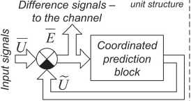
First, let us briefly explain the essence of the CGST method for processing arbitrary signals (Fig. 1). The system is excited by the vector of input signals, where T is the transposition operator. At the output of the coordinated prediction block, a vector of estimated signals is formed: U = (u 1, u2,..., uN)T. The system’s output is the vector of difference signals E (transmitting to the channel), defined as follows:

^-—^

E = U - U .

When receiving signals, transformations are carried out in reverse order: adding up the difference and evaluation signals allows us to obtain reconstructed signals, described as vector U (Fig. 1) as follows: — — ~

U = E + U .                                 (2)

signals from different channels during signal processing). In that case, an evaluation signal for a random channel number i can be defined as u i = W i • e i , where W i is the transfer function of the processing channel. In matrix form for an N -channel system without coordination with the same transfer functions for all channels W i = W :

'Ui ] (W 00

Ui2 = 0 wо u, [ 0 0 . W

I UN J XУ

( e i у

■

e 2

,

I ^eN J

Suppose there is no coordination in the described system (that is, there is no interchannel influence for

U = W ■ E ,                                 (4)

where W is the diagonal matrix of the transfer functions.

Compression

Estimated signals

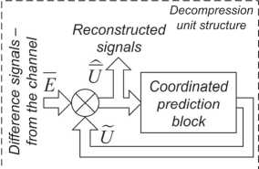
Fig. 1. The structure of the compression and decompression units with applying a coding matrix

Previously, in [22], we showed that the coding matrix CM could act as a coordinated prediction block in an effective coding system. CM describes as follows. The values of matrix elements k ij outside the main diagonal in rows and columns with numbers i , j ( i * j ) are calculated as correlation coefficients of signals from channels with numbers i and j ; the variable transmission coefficient K on the matrix main diagonal determines the compression ratio of the encoder and is specified separately according to the necessary compression ratio value. Thus, the matrix CM has the following form:

	■ K	k 12	..   k , .
CM =	k 2i	K	k 2 n	,                            (5)
	_ k m i	k m 2	•• K _

11N kij =      ■   E( Ui- Ui)( Uj- Uj),( I * J),          (6)

c i c J N^

and the vector of the evaluation signals U defines as follows:

.1“^..                                  -------

U = CM ■ E .

The compression efficiency of the CGST algorithm significantly depends on the correlations between signals of different channels [22]. The idea of our current work is that the color channels of an image are correlated because they describe the overall image. Fig. 2 illustrates the essence of applying CSGT algorithm for image compression. Input vector U in this case consists of the signals ur, ub, ug obtained from red, blue and green channels of the RGB image, respectively: U = [ur, ug, ub]T; the encoding matrix CM size for this case reduces to 3×3:

	■ K	к rg	kb '
CM =	rg	K	k bg
	_ k rb	k bg	K _

where k rb , k rg , k bg are the correlation coefficients between the signals of the image color channels, counted using equation (6), K is the variable transmission coefficient that determines the compression coefficient C [8], as it was mentioned earlier. At the second input of the comparimn element there is applied the vector U consists on signals u_r , u g , u b , generated by the coding matrix based on the vector of the difference signals E = [ e r , e g , e b ] ^T . The compression coefficient C is defined by the following equation:

C = SI size CI size , (9)

where SI size and CI size are the source and compressed images’ sizes in bytes, respectively. In decompression unit the decompressed image vector U is generated based on the vector E and the described coding matrix according to the Fig. 2.

2.    Testing the compression algorithm

We performed the simulation of the suggested compression algorithm based on CGST in a Python environment according to the Fig. 2. The performance of the described image compression algorithm was evaluated using the BSDS300 dataset [9]. It consists of 300 natural images and is commonly used for tasks in computer vision, such as edge detection, image segmentation, and object recognition

[10, 11]. The choice is caused by the necessity to evaluate the quality of reconstructing the original shades and object boundaries in the images. This dataset presents various brightness levels, color tones, and image sharpness, allowing for a comprehensive evaluation of the compression algorithm performance.

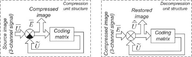
Fig. 2. The structure of the compression and decompression units with applying a coding matrix

We used the following quality metrics as the main performance indicators of the compression algorithm: Mean Squared Error (MSE), which measures the average squared difference between the pixel values of the original and reconstructed images; Peak Signal-to-Noise Ratio (PSNR), which measures the ratio of the maximum pixel value to the mean squared error; Structural Similarity Index (SSIM), which takes into account structural information of the image, including brightness, contrast, and the arrangement of gradient transitions; and Complex Wavelet Structural Similarity Index (CW-SSIM), a variant of SSIM that utilizes wavelets to analyze the structural information of the image, making it more robust to noise and distortions [12, 13]. Additionally, the processing time for each image was evaluated.

The algorithm was simulated for a three-channel system, with each channel corresponding to a color channel of the image. The value of the compression coefficient ( C ) was chosen to achieve compression ratios of 4, 6, 8, and 10. The results of the compression algorithm performance estimation for the different compression levels of the transmitted images are presented in Tab. 1.

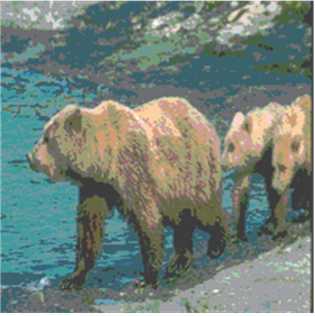
As the compression coefficient of the images increases, the reconstruction of the original image shades deteriorates due to the loss of correlation information between the channels. Additionally, with increased compression for each channel after quantization operation vast areas of pixels acquire the same brightness values that leads to undesirable images segmentation. Fig. 3, an example of such distortions in the output image is shown when using the CGST algorithm for the image compression.

Tab. 1. Average image reconstruction quality metrics for the original version of the compression algorithm when working with the BSDS300 dataset

Compression coefficient	MSE	PSNR	SSIM	CW-SSIM	Compression time, sec
4	23.69	36.35	0.97	0.95	0.73
6	34.08	32.35	0.96	0.94	0.73
8	71.19	29.61	0.94	0.93	0.72
10	90.19	28.58	0.88	0.91	0.71

a)

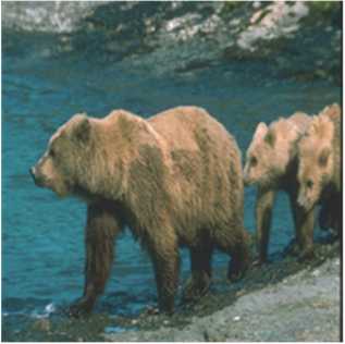
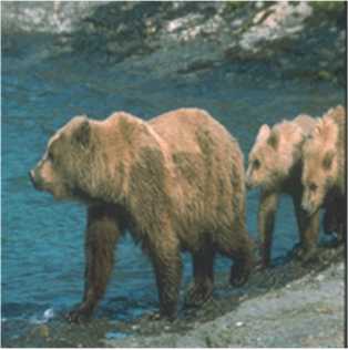
Fig. 3. Recovered images with compression ratios: a) 4 times, b) 8 times, c) 16 times

3.    Improving the compression algorithm

While testing the compression algorithm with the selected dataset, uneven restoration quality for half of the images was revealed. It is especially noticeable at low compression coefficients, at which the quality of the restored images is high. The most obvious indicator of this deviation is the MSE parameter. Based on the MSE average normalized value change over the whole dataset at compression ratio 4 (which provides high enough characteristics of the restored images), we divided the entire dataset into N1 set – with small MSE values and N2 set – with large MSE values. Fig. 4 shows MSE values for these parts with increasing compression coefficient.

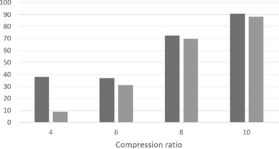
■ N2 N1

Fig. 4. Histogram of MSE values for N1 and N2 sets

MSE deviation at a low compression coefficient can significantly limit the suggested compression algorithm applicability. It was necessary to find a parameter characterizing two selected sets and a way to minimize the deviation of the algorithm’s image restoration quality indicator – MSE – for the whole range of images to solve this problem.

Based on visual analysis of sets N1 and N2, we put forward a hypothesis about the image frequency or its sharpness influence on the compression algorithm results. This assumption was partially confirmed by the difference in the spectrum pattern during the Fourier transform of these image sets. To analyze it, we generated three sets of primitive images with different frequencies of 300 examples each. These sets included gradient images, groups of pixels with similar tones, and geometric shapes on a homogeneous background, significantly varying in brightness and tone. Examples of these images are shown in Figure 5. Additionally, the compression time ratio with different image sets to the overall processing time was computed using the coefficients presented in Tab. 1. Tab. 2 shows the obtained performance metrics for these data.

The analysis of the results for reconstructing gradient images shows a gradual decrease in their quality as the compression coefficients increase. No significant deviation in MSE values was observed when processing this type of image at the same compression coefficients.

a)

b)

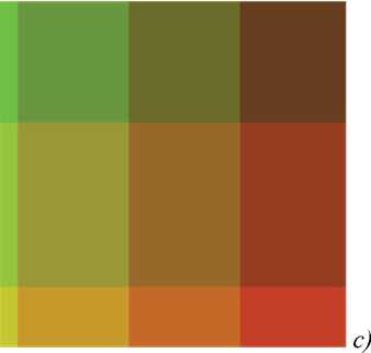
Fig. 5. Examples of generated images: a) gradient image, b) images with close-in-tone areas, c) image with figures on a contrasting background

Tab. 2. Average image reconstruction quality metrics for the original version of the compression algorithm when working with gradient images

Compression coefficient	MSE	PSNR	SSIM	CW-SSIM	Compression time ratio
4	11.57	37.49	0.98	0.97	0.82
6	18.41	35.47	0.96	0.83	0.98
8	72.78	29.51	0.9	0.75	1.2
10	92.55	28.46	0.9	0.76	1.3

Analyzing the results of the compression algorithm’s performance with tone-mapped images, the deviation in MSE values was most pronounced at a compression coefficient of 4, but it had a minimal impact on SSIM and CW-SSIM quality metrics. For compression coefficients of 6 and higher, this deviation was almost eliminated.

The analysis of image reconstruction metrics when working with shapes on a high-contrast background showed that the deviation in MSE values decreased at a compression coefficient of 6 and was almost completely eliminated only at a coefficient value of 8.

Based on the testing results of the compression algorithm on generated data, one can conclude that the magnitude of MSE deviations is most pronounced for images with frequent and high gradient transitions. The operating principle of the CGST method can explain this. The correlation coefficients between vectors formed from the image’s color channels were calculated for the image as a whole, resulting in incorrect correlation coefficients for individual image regions. The efficiency of the compression algorithm decreased due to the nonstationarity of the processed signals. In this case, it was logical to pre-segment the image into areas forming quasi-stationary signals. To achieve this, we performed the image segmentation on regions where the gradient varied weakly.

To separate these types of images, we used the Energy of Gradient (EoG) metric as a criterion. EoG allows for calculating the rate of intensity change across the entire image and provides a quantitative measure of high-frequency elements in the image [14]. EoG value E may be find as follows:

E =1 V fl² =

+

where Vfis the magnitude of the gradient vector, df/ 5x and df / dy represent the partial derivatives of the image intensity function with respect to the x and y coordinates, respectively, indicating how the intensity changes as one moves horizontally or vertically across the image. The normalized sum of EoG over RGB channels was calculated to analyze the images in this study. Images with smoothly changing gradients have the lowest EoG value; the highest value is characteristic of images with close-in-tone areas.

Tab. 3. Average image reconstruction quality metrics for the original version of the compression algorithm when working with tone-mapped images

Compression coefficient	MSE	PSNR	SSIM	CW-SSIM	Compression time ratio
4	68.08	29.8	0.97	0.99	0.97
6	23.48	34.42	0.95	0.92	1.06
8	54.63	30.75	0.95	0.96	1.15
10	86.9	28.73	0.90	0.87	1.22

Tab. 4. Average image reconstruction quality metrics for the original version of the compression algorithm when working with shapes on a high-contrast background

Compression coefficient	MSE	PSNR	SSIM	CW-SSIM	Compression time ratio
4	45.64	31.53	0.8	0.81	0.97
6	39.88	32.12	0.97	0.99	1.01
8	43.12	30.78	0.98	0.99	0.95
10	72.2	29.54	0.96	0.97	1

To verify the hypothesis regarding the influence of the gradient characteristics on the CGST-based compression algorithm efficiency, we calculated the EoG values for N1 and N2 sets. The average EoG values were 12.5 and 46 for sets N1 and N2, respectively. As shown in Figure 4, the MSE for set N1 was approximately four times lower. Thus, the EoG value for images can indeed be used as a metric for the non-stationarity factor affecting the algorithm’s performance. This parameter can be used as a criterion for dividing the original image into segments with a smooth gradient transition and correspondingly lower EoG. Both inter-channel and spatial correlations need to be considered to identify such regions. Therefore, the task at hand is a pixel clustering problem.

Due to strict requirements for temporal delays, the K-means algorithm was chosen for clustering, as it allows for the formation of clusters of similar pixels not only based on color and brightness but also in the image space [15]. However, the K-means algorithm requires setting a maximum number of clusters in advance. This parameter needs to be determined beforehand, considering that an excessively large number of clusters and the extraction of homogeneous regions will negatively affect both the clustering response time and the compression capabilities of the CGST-based algorithm.

It is possible to avoid excessive clustering through iterative selection of the number of clusters with a gradual decrease in their number from the maximum value to some threshold value. As a criterion for achieving a sufficient number of clusters, we can consider the derivative of the gradient function. Indeed, since we are discussing the necessity to achieve small gradient changes in each cluster, the criterion of such a condition fulfillment is zero equality of the considered function derivation. However, such a situation for all cluster points should indicate that the gradient is a constant value. From the point of view of the CGST operation, such a case is degenerate; the value of the correlation coefficient for the cluster equals one. During the simulation, we determined that a sufficient condition for MSE reduction is that the derivative of the gradient function in half of the points of each cluster under consideration is equal to zero.

This approach solves the problem of MSE deviation (non-uniformity for different types of images). However, it exacerbates the problem of high compression delay due to multiple iterations of clustering at initially high values of the maximum number of clusters. These operations also introduce unnecessary computational complexity. Therefore, a method is needed to determine the required maximum number of clusters for the K-means algorithm based on the characteristics of the original image, minimizing the image reconstruction MSE parameter without introducing significant temporal delays.

Machine learning algorithms, such as classical neural networks, have a high potential to solve many optimization problems without adding significant delays (for a small number of input parameters) [16]. Since, in this context, the neural network is used for regression, and there are high requirements for its response time, the choice was made in favor of Radial Basis Function Networks (RBFNs) [17] due to their high potential in approximation tasks, relatively low response time, and time required for retraining. The latter provides some potential for using this structure in non-stationary systems. The combination of RBFNs and K-means enables the implementation of adaptive clustering, taking into account the characteristics of input images.

Iterative learning was employed as the chosen approach for training the RBFN to simulate the compression algorithm’s operation. The compressed image, 32 by 32 pixels in size, was fed as input to the RBFN. Processing this input does not require high computational complexity while preserving brightness and spatial information. The output of the neural network represented the maximum number of clusters, which was then provided as input to the K-means algorithm during the reception stage without conducting clustering.

The error function during the RBFN training process depended on the MSE of the reconstructed image. The number of neurons in the hidden layer was determined based on the system’s performance requirements, aiming for no more than a 30% increase in processing time compared to the original CGST-based compression algorithm version, while reducing the average MSE level by over 20% for a compression ratio of 4. These requirements were satisfied by the RBFN structure with 100 neurons in the hidden layer. The results of the algorithm’s operation with adaptive clustering are presented in Table 5. Figure 6 shows the effect of suggested CGST improvements on MSE deviation for N1 and N2 sets for the compression coefficients 4 and 6. Based on the obtained data, the application of adaptive clustering helped to reduce the average MSE value of the algorithm’s operation by more than 25 % and decrease its deviation by over 40 %.

Tab. 5. Average quality metrics of image recovery by the original version of the compression algorithm with clustering over the whole dataset

Compression coefficient	MSE	PSNR	SSIM	CW-SSIM	Compression time ratio
4	17.5	37.04	0.97	0.96	1.3
6	32.56	32.97	0.96	0.94	1.28

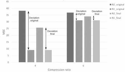
Fig. 6. Histogram of MSE values for N1 and N2 sets with adaptive clustering

4.    Discussion and conclusion

In this work, we showed that it is advisable to supplement the CGST-based image compression algorithm with preliminary image clustering to improve its effectiveness and remove restrictions on the CSGT for compressing images with high EoG values. This approach allows applying CGST to each image area the clustering algorithm selects, and this may also improve other image compression algorithms sensitive to the images’ characteristics instability. For example, computer vision algorithms are sensitive to linear and nonlinear changes in the spatial intensity of images [23]. In turn, the intensity of the image gradient significantly affects the change in spatial intensity and visual quality of the image [24, 25], and, accordingly, the complexity of detecting image patterns by machine learning algorithms.

Applying RBFN helped us significantly speed up the clustering process. The delays added by the described compression algorithm do not yet allow it to be used as a video codec for systems that provide users with video streaming services or other systems critical to delays. However, the proposed approach may be effective for many IoT systems processing multimedia data. For example, in medical Internet of Things systems, when conducting endoscopic examinations ([18, 19, 20]) or remotely examining a patient using telemedicine systems ([21]), the requirements for reducing the WSN load and increasing its nodes’ battery life come to the fore. The algorithm we described allows us to provide at least fourfold additional compression of images processed by existing compression methods while maintaining acceptable quality of reconstructed images according to the criteria MSE, PSNR, SSIM, and CW-SSIM. At the same time, the described algorithm can also provide high compression ratios for systems in which deterioration in image quality is acceptable while maintaining their overall information content, for example, in video surveillance systems or emergency monitoring.

Acknowledgments

The research was supported by Russian Science Foundation, agreement No. 21-79-10407 (mathematical model), by the Ministry of Science and Higher Education of the Russian Federation: state assignment for USATU, agreement № 075-03-2021-014 dated 29.09.2021 (FEUE-2021-0013) (algorithm adaptation), and by the Ministry of Science and Higher Education of the Republic of Bashkortostan, agreement №1 dated 28.12.2021 (simulation and analisys).