Approximating Spline filter: New Approach for Gaussian Filtering in Surface Metrology

Published Online October 2009 in MECS

In conventional surface metrology, surface assessment is always on profile as the curve of intersection. In recent years, with improvement of manufacturing techniques and demand of quality control, three dimensional (3D) analysis of surface geometry has become more and more important. Thereunto, mean line is the reference line about which the profile deviations are measured, mean surface is the 3D reference surface about which the topographic deviations are measured[1]. Both the mean line and mean surface is established by applying a filtering process to the measured surface. Filters selected in this establishment have become critical for numerical

Manuscript received January 18, 2009; revised June 19, 2009; accepted August 22, 2009.

characterization and parameters determination.

The profile filter of Gaussian is the most widely used filter described in ISO11562 [2], [3]. Gaussian filter is superior to 2RC filter by two advantages, phase-corrected property, which is a simpler way to employ by many fast algorithms [4],[5]. However conventional Gaussian filter has indelible end effect, even the GR2 haven't resolved it entirely but with larger computation cost [6]. In fact, according to the point of view in digital processing, convolution is the primary reason of end effect. The output data are the convolution results between the filter transfer function and input data, then the end effect generates during this process.

In order to overcome end effect, Krystek proposed a new spline filter algorithm to substitute for Gaussian Filter [7]. This method adopts numerical fitting and matrix equation solution to obtain the mean line, with result in abandoning the filter's convolution [8],[9]. T.Goto proposed the robust spline filter which is less influenced by outliers and also implemented through matrix equation [10].

Both of them can obtain a kind of mean line to analyze the surface profile. These filters are all designed for overcoming certain limitations existing in the surface measurement such as end effect, computing efficiency and robustness. However, they, besides Numada [11], all overlook the most important thing, which is the substitution likelihood for ISO standard of Gaussian. Above all, Gaussian filter is the ISO11562 standard with a distinguishing feature of at least space-frequency product whose cutoff is sufficiency for profile filter. How to not only preserve Gaussian filter's transmission characteristic, but also restrain end distortion becomes a stubborn problem.

In this paper, the new kind of spline filter which not only inherits the ordinary spline filter quality but approximates to Gaussian filter is brought forward. i.e., in bosom of measured data, the filtering results conform to the ISO standard, at the same time, the end effect is restrained by numerical fitting technique. In addition, to 3D surface evaluation including enormous amount of computation due to large quantity of sampling data, it also yields a fast filtering process.

• II.    Approximating spline filter

The spline filter based on variation differential theory had been proposed by Schoenberg[12] and Reinsh[13] for 50 years. Poggio applied to the variation spline of Tikhonov, regularization to image process and stated it as leading to a Gaussian-like convolution filter[14],[15]. Given a set of measured value sampled z_k , the spline filter is defined as the function:

Л d m (()\ 1 ²

• ^е = У { z k ^{- 5 (} x k ) } + M N л m Г ^dx ^ ^Min (1) k = 1                           I dx J

where k is the index for the sampled data, s ( x_k ) is the output data, n is the number of measured points, ц is the LaGrange constant, 2 m - 1 is order degree of spline. The differential order m is higher than the spline filter cutoff is more steplike [16]. Actually, in ordinary condition of convenient calculation, m is given 2, and the spline is cubic order. This spline definition can be thought as the compromise between approximation to data and bending energy of spline through ц constant. The functions are discussed in this literature considering the general case of equally spaced nodes and a finite number of input data, for the natural condition of measured profile data.

In order to resolve the problem of end effect existing in filtering results by Gaussian filter, the spline filter has been proposed for profile measurement [8]. However, these spline filters differ greatly from Gaussian transmission. In fact, for digital instruments, excluding disadvantage of end effect, Gaussian filter is appropriate filter for surface profile evaluation, and sufficient to separate profiles into long wave and shortwave components. Therefore, (1) is expected to be reconstructed to perform better realization of Gaussian filter. In Johannes’ paper [17], a first order differential is added into the second item of (1) to achieve this pursuit. So a new type of spline filter named approximating spline filter in this paper is constructed. The approximating spline filter is expressed by

/ a2 f I1 d 5 ( X ) |

{ zk - 5 (xk )} + M Hl~I + k=1                    К dx )

( d5 (x) VI т|-----I Гdx ^ Min           (2)

У dx ) J where т is the Gaussian approximation coefficient. Regulating т properly, the solution of (2) can be close to the result filtered by Gaussian filter, and (2) can be named the spline realization of Gaussian filter.

Adapting to digital processing, (2) must be discretized as the following equation:

nn e = Уzk - sk}2 + M^{(v2sk)2 + т(Vsk)2} ^ Min k=1

where V is the difference operator[16], and

m

V msk =Z{(-1yCm • St+L m/2j_i } i=0

where C_mⁱ are polynomial coefficients.

To achieve the minimum of function (3), an equation similar to partial difference with respect to s_k is implemented by

^= о d s_t

There are two types of boundary conditions, which are the non-periodic data and periodic data [10], thereunto, the former is also called nature boundary condition. Depending on the different boundary conditions, we can deduce different filters that also adapt to different tasks. For most instances, engineering surfaces possess arbitrary and non-periodic distribution, for which the nature boundary condition is needed, that is

V ² 5 1 = V 2 5 n = 0 (6)

Utilizing equation of (5) and (6) ， the following equations are constructed:

d e

— = -2(z 1 - 51) + 2ц{S3 - (2 + т)52 + (1 + т)51} a5

-- = -2(z2 - 52) + 2ц{54 - (4 + т)53 + a52

(5 + 2 т ) 5 ₂ - (2 + т ) 5 1 }

<        f ^- = - 2( z_k - 5 k ) + 2 m (V⁴ 5 k - f V ² 5 k )         (7)

a5k de

7--- = -2(zn-1 - 5n-1) + 2ц{5n-3 - (4 + т)5n-2 + d5n-1

^{(5 + 2 т} ) ⁵ n - 1 ^{- (2 + т} ) ⁵ n }

• I ^-    = ^{- 2(} z n ^{- 5} n ) ⁺ 2 M { ⁵ n - 2 ^{- (2 + т} ) ⁵ n - 1 ^{+ (1 + т} ) ⁵ n }

У ⁵ n

For some special cases such as calibration specimens, their surface present strongly regular and period distribution, and such a surface should be disposed with period boundary condition as shown as:

⁵k = ⁵k + n ⁽⁸⁾

Hence, it introduces another partial difference equation by (5) and (8)

I ^- = - 2( z_k - 5 k ) + 2 m ( V ⁴ 5 k - 7 V ² 5 k ) = 0       (9)

a ⁵ k

We observe that both (7) and (9) can be written as a kind of uniform matrix equation such as:

( I + M Q ) S = Z                 (10)

where I is identity matrix, Z is the vector of measured data, and S is the output result data. Q is well-deduced coefficient matrix, with (11) and (12) corresponding to the nature boundary

condition respectively.

⁴ 1 + т - 2 - т    1

condition and period boundary

1 - т	1			(11)
- т	6 + 2 т	- 4 - т	1
1	- 4 - т	5 + 2 т	- 2 - т
	1	- 2 - т	1 + т

6 + 2 т

- 4 -т

Q =

• -4-т    1                     1

6+2т -4-т    11

• -4-т 6+2т -4-т1

1    -4-т 6+2т -4-т1

1     - 4 -т 6 + 2 т - 4 -т

1                     1     - 4 -т 6 + 2 т _J

III. Approximating coefficient

The weighting function and transmission characteristics of Gaussian filter are given by ISO11562[2]:

h ( t ) = — e -' ⁽ t / ^aA c )² aA c

H ( A c I A ) = e - * ^{( аЛ} с / ^A

where a is a constant, , A is wavelength , and A c is cut

off wavelength. When A = A c , the filter has 50%

transmission, then a = 0.4697 . “It is of importance that the transmission for the cut-off wavelength is 50% since the short wave and long wave potions of the surface profile are separated and can be recombined without altering the surface profile[2]”

The transmission characteristic of the approximating spline filter has been derived from (9)[17]:

zk = A s k - 2 ^{- (4 + т} ) A s k - 1 ^{+ (1 + (6 + т} ) A ) s k ^{- (4 + т} ) A s k + 1 ⁺ A s k + 2

Using the Z-transform, we get 5 ( z ) = G ( z ) Z ( z ) , with Z ( z ) the Z-transform of the sampled data z_k and S ( z ) the

Z-tansform of the solution data s_k and with filter G(z) is

given by

G ( z ) =

A ( z ² + z ²) - (4 + т ) a ( z ^- + z ) + 1 + (6 + 2 т ) A

Substitution of z by exp( - j m ) in G ( z ) yields the discrete Fourier transform G ( m ) of this regularization filter

G ( m ) =

1 + 2 та • (1 - cos m ) + 4 a (1 - cos m )²

In (13), there are many different approximation forms to Gaussian filter obtained by different value т . Our purpose is to find a knowable expression as an optimal choice. `”The closest approximation to the Gaussian function Fourier spectrum is obtained in the case of т = 11 JA [17]”. In addition, it is obviously reduced to ordinary spline filter when т = 0 .

We have known that the Gaussian filter has 50% transmission characteristic in the cut-off frequency, this requirement is also been adopted to spline function, that is

1 + 2T A • (1 - cos m _c ) + 4 a (1 - cos m _c )²

¹₂       (14)

For spatial signal, the digital angle frequency m = 2 n d I A , d is sampling interval which is assumed unit value in this paper for convenience, and A = n . When A = A c ,

^m c

2n nc

From (14) and (15), LaGrange constant a can be derived by

_________________1_________________= 1

1 + 2T A • (1 - cos —) + 4 a (1 - cos — )^{2  2}

ncnc

It's observed that (16) is a quadratic equation in one variable with respect to T A , therefore, a can be solved

as

A = ⁽^ " ¹⁾² .                    (17)

64sin⁴ 1 —

I n c J

From this A , as shown as Fig.1, the frequency amplitude of an approximating spline filter matches with that of Gaussian filter well. Fig.4 shows that the maximum of the amplitude deviation between approximating spline and Gaussian is only 4.26%, which is even less than many Gaussian filter simplified algorithms. On the contrary, the maximum of amplitude deviation between ordinary spline and Gaussian filter is 10.6%, which is illustrated graphically in Fig.2. So it is clear that approximating spline, not original spline, is selected as the approximation to Gaussian filter.

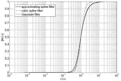
Figure 1. Transmission characteristics of digital filters.

Approximating spline has no phase shift error, because the odd order spline is symmetry to a vertical axis whose property is the same as Gaussian function, and even order

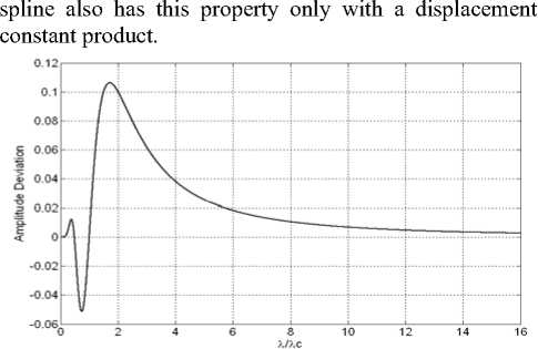
Figure 2. Deviation of transmission characteristics.

• IV. Cascades of approximating spline filter

For some special conditions, approximation with 4.26% deviation isn't enough for practice. This filter algorithm must be improved to fit higher accuracy Gaussian results. If single step of approximating spline filter is regarded as a basic process prototype, quadratic cascades of them can attain better approximating effect. In these situations, ц must be recalculated, because the quadratic algorithm should also stand by 50%. The quadratic algorithm is constructed as

G( о ) = [ 1 + 2 тц • (1 - cos о ) + 4 ц (1 - cos о )² ]      (18)

The approximating coefficient and lagrange constant are also calculated by the method introduced, the similar as (17) in previous section, but

( 7472 - 3 - 1 ) 2 ^ц =-----

64sin⁴ I ^— I

I n=)

and т = 1/7 ц as of old. In Fig.3, amplitude transmission between the quadratic cascaded approximating spline and

Furthermore, if n cascaded spline filter is executed, the transmission function is defined as

G ( о ) = [ 1 + 2 тц • (1 - cos о ) + 4 ц (1 - cos о )² ]        (19)

where

(7 4 72 - 3 - 1 )

ц =^-------(20)

64sin⁴ 1 ^— I

I n c )

It's found that if the spline order n is more higher, the approximation deviation between multiple approximating spline filter and Gaussian filter is more lower, that is, when n ^ да , this spline filter approaches Gaussian transmission characteristic infinitely. In Fig.4, the 30 cascades can approximate to Gaussian filter with fluctuant but maximum 0.52% deviation.

Fig 5 shows this approximation trend for each cascading order spline through 1 to 500, in which the maximum approximation deviations are almost under 1%, except order 1 and 3 to 11, and generally incline to zero. The stricter explanation of this trend is referred to central limit theorem [4]. From above analysis, it is turned out

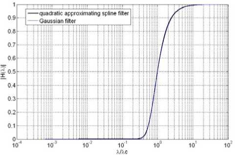
Figure 3. Transmission characteristics of digital filters.

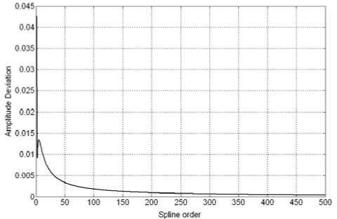
Figure 5. Approximation deviation of each cascaded spline filter.

Gaussian filter is compared, and the maximum deviation depicted in Fig.3 between them is 0.92%. This result is considerable satisfying compared with relative deviation tolerance (-5% ～ +5%) in ISO11562. See Fig.3, their transmission characteristics is superposition each other ultimately.

that quadratic cascaded approximating spline filter is the optimal choice compromising between efficiency and precision.

V. Two dimensional filter

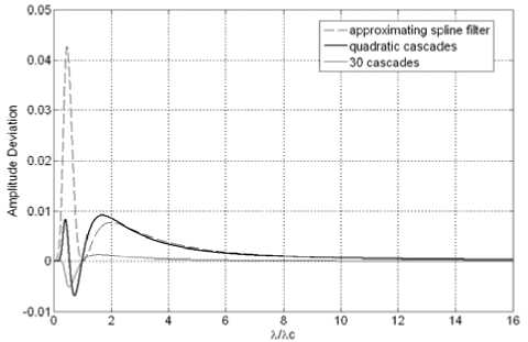
Figure 4. Deviation amplitude between approximating spline filter and

3D surface analysis presents the geometrical form of an area on a work piece more particularly than the profile of 2D. The mean surface, similarly to mean line for profile, established by the form filter, is a reference surface for 3D surface evaluation. A roughness surface is obtained by subtracting the mean surface from the primary surface.

Extending the weighting function of Gaussian filter to 2D, we obtain the 2D Gaussian filter for 3D surface measurement

h ( x , У ) =

P^- XC ^ yc

• exp <

— в

whose transmission characteristic is given as

H( A x , A y ) = exp <  -пв

where Axc and Ayc is the cut-off wavelength along x axis and y axis. When Ax = Axc, Ay = * or Ay = Ayc, Ax = « , the amplitude transmission is appealed for 50%, then в = ln2/п .

In general, (22) can be reduced to the product form of two independent Gaussian filters:

H ( A x , A y ) = exp \-в

n { Ayc)

• exp ^ - пв | ^- I f

= exp <

= H ( A x ) • H ( A y )

which clearly indicates that it is a simple realization of 2D Gaussian filter and that it can be achieved by employing two 1D process to x-coordinate and y-coordinate respectively.

The 3D surface evaluation, the total number of pending data is so enormous that original spline filter requires maximum of 1h for computation, hence, we should pay more attention to the implementing of efficient processing algorithm [16]. On the other hand, the data corresponding one direction section of 3D is downsampling generally in contrast to profile, it need to alleviate the end effect more necessarily for preserving limit valid data. Here, we select the 2D approximating

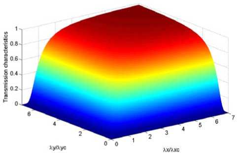
Figure 6. The transmission characteristic of 2D approximating spline filter.

spline filter as the form filter to extract mean surface. The similar to 2D Gaussian filter, a 2D approximating spline filter can also be obtained by extending respectively two 1D approximating spline filter along x-direction and y-direction, whose results are composed for a whole 3D reference surface. According to above discussion, we have known the approximating filter can approximate to the transmission characteristic of Gaussian filter with admissible tolerance. The 2D approximating spline filter can also approach the 2D Gaussian filter with high accuracy.

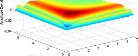
Fig. 6 shows the transmission characteristic of 2D approximating spline filter of quadratic cascades. Fig.7 describes the deviation between the 2D approximating spline filter and Gaussian filter, the deviation is limited in -0.63% □ + 1.48% , which is acceptable outcome for most assessments of 3D surfaces.

• VI.    The algorithm

In previous sections, we present the configuration of approximating spline filter, and explain the approximation property with Gaussian filter particularly, in this section, an efficient fast algorithm to implement approximating spline filter will be introduced. Observing (10), it is distinctly that this filter algorithm to profile data will be solved by matrix technique, which is discussed by three step as follows:

• a)    Compute ц by (17), and defined ( I + ^ Q ) = Q . Q as still a positive definite matrix and diagonal dominant.

• b)    Q ^' can be disposed based on Cholesky decomposition. Q = R T DR , then R T DRS = Z .

• c)    Assuming DRS = Y , the algorithm can be divided into R T Y = Z and RS = D ^{- 1}Y .

• d)    If cascaded algorithm needed, repeat step c) with designed cascaded order iteration, else end. Note ц is calculated depend on the cascaded order by (20).

8 0 02.

It has related that 2D filter for 3D surface evaluation can also be realized by this spline filter, who will perform respectively the algorithm related above along the x-coordinate, then along x-coordinate in successive order, and achieve the approximating results to 2D Gaussian filter.

In fact, this algorithm is similar to Krystek's[7]. This algorithm denotes a complete matrix calculation without the convolution between data and discrete filter, and doesn't need a data preparation stack. Therefore there is almost no end distortion during this process. This good property will be testified by the experiments of next section.

0 041

xx/Xxc

Figure 7. The deviation between the transmission characte r istics of approximating spline filter and Gaussian.

• VII.    Experiments and discussion

In order to validate the characteristics of approximating spline filter, in this section, some experiments are conducted to extract reference lines or reference surfaces toward real profiles and simulated surface.

• A.    Mean line

  A real work piece profile is measured and data points are sampled. The total length is 5.6mm, and sampling interval is 0.5 ц m, then 11200 digital points are obtained. Quadratic approximating spline filter with nature boundary condition is applied to these points for mean line with 0.8mm cutoff wavelength. As shown as Fig.8, the mean line extends smoothly along the general tendency of real surface.

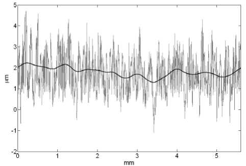
Figure 8. Profile data and mean line with X _c = 0.8 mm .

As a comparison, we also apply this filter to a sequence data of period signal, which has sine wave distribution texture. Fig.9 shows sine profile and the extracted mean line, which indicates the period boundary condition in this case, preserves the filtering end better than nature boundary condition.

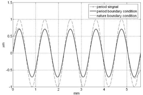
Figure 9. Profile data and mean line with X _c = 0.8 mm .

All of above algorithms are programmed elaborately using Matlab language and executed on Pentium dual E2140 1.6GHz machine with 1G EMS memory, its computation cost for once extraction is only 4 ~ 8ms.

• B.    End Effect

In Fig.10, Both Gaussian filter and quadratic approximating spline filters are employed for mean line. In the midst of the results, mean lines extracted superpose

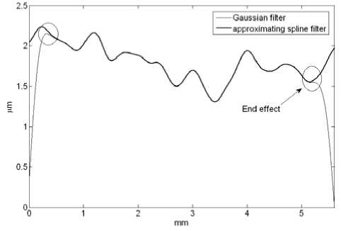
Figure 10. Comparison of performance between Gaussian and approximating spline filter.

each other. This fact testifies the feasibility of spline realization for Gaussian filter furthermore. In addition, the results of Gaussian filter have large distortions on both ends. However, approximating the spline filter is influenced little by these distortions. From this experiment, it demonstrates that approximating spline can extract mean line from original data reliably and restrain end effect at the same time.

• C.    Mean Surface

Before performing a 3D surface experiment, we introduce a simulated surface which is constructed by fractal theory. It is confirmed that many surfaces have a fractal geometry within a certain scale range [18]. Roughness measurements on processed surfaces show that rough surfaces are composed of both brownian and non-brownian spectra at various length scales [19]. It is also understood that a rough surface which exhibit statistical resemblance to real surface can be simulated by Weierstrass-Mandelbrot (W-M) fractal function deterministically, as follows:

z (x, y) = F (D) A(D-1) x where

Ю z n = n

cos 2 ny ⁿ { x + g ( y ) } cos 2 ny ⁿ { y + g ( x ) } Y (²- D ) n

1/2

I (25)

( 2ln y (5 - 3 D )(7 - 2 D ) E ( D )

F(D) = I--------------------------- V           n and E(D) is an integral

E ( D ) = j { cos^{(5 - 2 D} ) в - cos⁽⁷ ”^{2 D} ) 0 } d e          (26)

Note D is the dimension of a profile whereas the dimension of the surface is Ds = D +1, (1< D < 2) . The frequencies Yn of W-M function form a spectrum ranging from Yn to infinity in geometric progression. The parameter Y determines the density of the spectrum and the relative phase differences. The function g(a) is introduced to randomize the phases such that for each value of y the profile along x has different phase and vice versa [19].

Equation distribution

^∞ cos2 πγ ⁿa g ( a ) = C ∑    _{(2 - D ) n}                  (27)

n = n ₁ γ

(2 - D )( n 1 - 1)

C = ^{1 γ}                    (28)

2 _× 2^1/2 _{ γ (4 - 2 D ) _- 1 _} ^1/2

• (2 7) illustrates signal of a Gaussian

with standard deviation σ . If the random phases vary between π and -π, then σ = 1/4 . Provided γ = 1.5 , Fig.11 produces a simulated surface with 2000 × 2000 points deduced by (24).

Finally, the 2D approximating spline filter is used to extract mean surface of simulated fractal surface in order to verify the practical effect. The cut-off wavelengths of

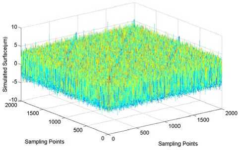
Figure 11. Simulated surface.

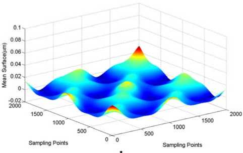
Figure 12. Mean surface.

λ _xc and λ _yc along x-axis and y-axis is respectively defined 400 sampling intervals. Fig.12 shows the mean surface and proves this filtering result has a smaller evaluated end effect, this is thought to be because the alleviation ability of nature boundary condition to the distortion of end points. Furthermore, it is accounted the total processing is completed in less than 2.3s.

VIII.    Conclusion

A new spline filter for profile measurement is developed, and its characteristics are detailed, which is just defined as approximating spline filter to differentiate from ordinary spline. This spline filter inherits the smoothness and no-end-effect of ordinary spline. The most important property is its Gaussian approximation, and amplitude deviation of approximation only achieves 4.26%. When quadratic cascaded approximating spline carried out, the deviation is reduced to 0.92%. Therefore, for domain of the surface metrology, approximating spline filter is regarded as the spline achievement for Gaussian profile filter. In addition, 2D filter can also be composed of these spline filters to process 3D surface, and this 2D filter can approximate to Gaussian filter with accepted deviation -0.63% □ + 1.48% . Thank to matrix decomposition algorithm, this filter algorithm has high speed computation, working on a general computer, its total execution processes for 11200 profile points, and 2000 × 2000 surface points only spend about 8ms and 2.3s respectively.