Asymptotic Stability Analysis of E-speed Start Congestion Control Protocol for TCP

Published Online May 2012 in MECS

Window based congestion control has been widely studied and a large number of protocols have been proposed in literature. In general, window based congestion control has four states, these are slow start, congestion avoidance, fast recovery and fast retransmit. Two important algorithms of the window based congestion control are the slow start and congestion avoidance. Congestion avoidance algorithm has been modified severally by a great number of researchers and many advances have been made to TCP [1], [2] , [3], [4] , [5], [6], [7], [8], [9], [10], [11]. The attention of the network research community has recently focused on other aspects of congestion control such as the slow start and acknowledgement congestion control. Proposals to modify the slow start include SPAND by [12], and Swift Start by [13-14], Limited Slow Start [4], Restricted slow start by [16], Quick Start by [17], P-Start by [18] Capstart by [19].

In this papaer, a multiple start-up for window based congestion control (E-speed start) is being proposed. Espeed start specifies that TCP transmission speed be selectable from several possible startup speeds depending on the prevailing network condition, instead of a single startup for TCP as specified by the current window based algorithms. This concept can be extended to an n-arry selectable startup speed for window based congestion control protocols.

The remaining part of the paper is organized as follow: section II discusses the E-speed start mechanism, section III introduces the concept of utility maximization and thereby derives a model for E-speed start. In section IV, the stability of the derived model was proved, and section V concludes the paper.

• II.    E-SPEED START MECHANISM

• 0. Estimate the value of β using available bandwidth. If β=1 go to (1) else if β>1 go to( 8)

In e-speed start mechanism, new connection starts with TCP sending an initial packet. Thereafter, the congestion window is grown by;

cwnd = 2n β                      (1)

This is a modification of maximum window size per cycle of slow start where n is the number of RTT and β is a function of the available bandwidth. If β is set to one, transmission proceeds via the traditional slow start and one additional packet is transmitted in response to one ACK (packet acknowledgement) received. If β is set to two, then four packets are sent per each ACK received and it continues until there is a notification of congestion with each ACK received, E-speed start adds 2β – 1 packets to the current window size. i.e. for each packet received cwnd=cwnd+2 β – 1           (2)

Equations 1 and 2 form the bases for the window growth function in the E-speed start. It is important to emphasise here that network capacity utilisation is the main trust of the E-speed start algorithm. The algorithm can adapt its speed from network to network hence it is both backward compatible with networks with low bandwidth delay product (BDP) and forward compatible with networks of higher BDP.

The e-speed Start Algorithm

• 1.    Start with a window size of 1 i.e cwnd=1

• 2.    Increase the window size by 1 i.e. cwnd=cwnd+1;

• 3    for every ACK received, repeat step (2) until the ssthresh is reached OR packet loss is detected

• 4.    If ssthresh is reached, go to (7).

• 5.    Else If a packet loss is detected, go to( 6)

• 6    set to ssthresh = 0.5*cwnd set cwnd =1 go to step(2)

• 7.    Exit (transit to congestion avoidance)

• 8.    Increase the window size by 2^β-1 i.e. cwnd = cwnd+2^β-1; for every ACK received. Repeat step (7) until ssthresh is reached OR Packet loss is detected

• 9.    If ssthresh is reached, go to (7)

• 10.    Else if a packet loss is detected, go to (6)

This function i.e. equation 1; is a more aggressive and somewhat friendly approach. The growth in the congestion window by this function gives a greater utilization of the available bandwidth in very good time. If the congestion window is opened more aggressively at the slow start stage, without proper consideration of the state of the network before embarking on probing the network, it might lead to an instance of congestion collapse or TCP fairness could be reduced to the minimum as other TCP variants on the network may be marginalised in the share of the available bandwidth. Although full utilization will be achieved, there will be greater vulnerability, as a congestion collapse might just be a round trip time away. This completely rules out the reason for the invention of the Transmission Control Protocol. Most high speed TCP variants maintained the slow start while some aggressively open up the congestion window only during steady state that is, during the congestion avoidance state observed in standard TCP. Below is a comprehensive analysis of the proposed algorithm.

• III.    E-SPEED START MODEL ANALYSIS BACKGROUND

  Prior to 1997, when [20] introduced the Kelly’s system problem, researches in congestion control was intuitive, based on laboratory experiment, simulation and validation, but with the Kelly’s paper in [21] titled “Rate control in Communication Networks” The research community began to model congestion control mathematically. There has been a vast research effort in this area. Currently, research activities in this area has produced quite a number of models as seen in literature. One important research direction is the search for better understanding of how today’s Internet works.

Jacobson’s Additive Increase and Multiplicative Decrease (AIMD) algorithm [22] has worked so well on the Internet which has metamorphosingng from a few number of users to a giant networks with millions of users worldwide. However, the adequacy of these models has been questioned by many researchers in today’s and future Internet traffic which is changing rapidly in nature. The rapid growth in traffics of multimedia application protocol, voice over Internet(VoIP), video conferencing, games etc. which use protocols that are quite different from TCP has made the current internet an interesting area of research. While TCP is self-regulating in the face of congestion, these other protocols are quite aggressive and hence fairness in the sharing of bottleneck links is not encouraged. Therefore, mathematical models of congestion control are being proposed in literature. [23] classified models for congestion control and related tools as packet-level models, fluid flow models and hybrid models.

A packet-level model accounts for the location of each individual packet as the packets are queued and forwarded through the network. The system state evolves as a series of discrete events. The events in Internet are arrival and departure of packets, and timeouts. A fluid flow model sees the data transport as a continuous fluid, with no packet boundaries. State variables vary continuously, and are described using differential equations. In congestion control, fluid flow models do not capture all details of the dynamics. Instead the state variables represent averages of the true system state. Here, evolution of the state is a result of discrete events together with continuous changes between events. A continuous model is used for queuing dynamics and endhost actions while action like multiplicative decrease of TCP is modeled as discrete event. The pioneering work of Kelly [20] on network utility maximization has spurned a great research interest in mathematical analysis of internet congestion control.

• IV.    APPLICATION OF NETWORK UTILITY MAXIMIZATION TO E-SPEED START

The network utility maximization framework enables investigation into properties of networks. Prior to this time, modeling techniques available allow for analysis of small networks with a high level of mathematical complexity.

The global optimization problem which maximizes aggregate utility as formulated by [21] is:

Max ^U n ^{( x} n ⁾

Subject to Rx <  c

Where c is the link capacity, ^x n are the source transmission rate and R is the routing matrix R _ln .

x=(x 1 , x 2 , x 3 , . . . ,x n )^T,

Vector inequalities are element-wise.

The capacity constraints Rx <  0 and x >  0 defines a convex set. If ^U n ^{( x} n ⁾ are concave functions, then the utility maximization problem is a convex problem and thus has a unique solution. According to [24-25], convex problem can be solved using Lagrangian Method.

The AIMD uses decentralized end-to-end principle and a centralized solution to the utility maximization problem is not in line with the end-to-end principle. Hence a decentralized solution is sought for the utility maximization problem. Introducing the Lagrangian function to the utility maximization problem

N

L ( x , p ) = ∑ U_n ( x_n ) - p ^T( Rx - c )

n = 1

N

= ∑ U_n(x_n) - xR^Tp+p^Tc n= 1

N

= ∑Un(xn)-xTq+ pTc n =1

NN = ∑ ( U_n(x_n) - x_nq_n)+ ∑ p_lc_l           ( ³ )

n= 1                             n= 1

Where q=RTp is the aggregation due to routing

The dual problem is given by

Min Max L(x,p)

p ≥ 0, x ≥ 0 where p is vector of langragian multipliers Let (p*,x*) be the primal solution to the dual problem, convex duality implies that (p*,x*), is the solution to the primal utility problem. The dual problem is given by

NL

Min ∑ Bnqn + ∑ plcl(4a)

n=1

where Bn(qn) = Max Un(xn) – xnqn(4b)

Eq. 2 can be interpreted as maximization of individual sender’s profit where q n is the price it is charged per unit flow. Note that in this context p l can be seen as price charged by link l per flow.

The transformation of (3) into (4a) and (4b) enables a decentralized solution as the availability of price q _n to source n will make the solution of (4b) possible without requiring other sources rate. Also p*, when aligned with langrage multipliers and compute in a decentralized manner by sender will also find a solution to the utility maximization problem because of convex duality [26].

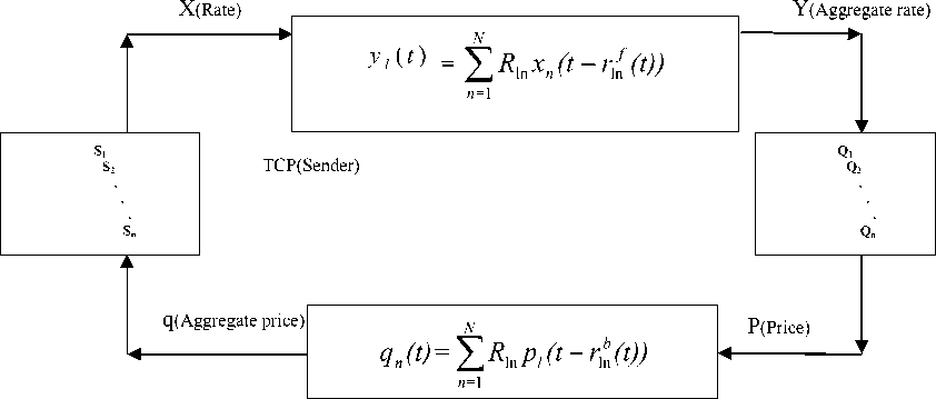
Next, a model is formulated for E-speed start using TCP New Reno model and modifying it for the slow start and thus devising the E-speed start model. The general network model is described in figure 1; Let define the following;

x_n ( t ) y_l ( t ) p_l ( t ) q_n ( t )

- source n transmission rate

- link l aggregate incoming flow

- congestion measure for link l or price for link l

- aggregate price for all links w n (t) - window size for source n rn (t) - round trip time of source n a network is modeled as a set of links L with finite capacity c l , ( l ∈ L ). These links are used by N sources transmitting data at rate x n ( n ∈ N ). Each source n uses a subset Ln ⊆ L of links. The sets L n define an L × N routing matrix

R = { 1     iε L ln 0       otherwise

Each row of matrix Rln defines each link in the network while each column defines each data flow. A data flow consists of source node, destination node and sending rate. We shall assume that the destination node is passive hence a source refers to the source node and its sending rate. Let the sending rate of a source n be xn (t)

The relationship between the window size sending rate is given by:

Sending rate = Window size/ Roundtrip time and the

x_n ( t ) =

w_n ( t ) r_n ( t )

Each link l has an aggregate incoming flow rate yl (t) . Propagation delay consists of both forward and backward delays: denote by rln f (t) the forward delay and rln (t) the backward delay of source n and link l.

Then, the aggregate flow rate at link l, ^y l ^{( t )} is given by

N yl(t) = ∑ Rlnxn(t - rlnf (t)) (6) n=1

The congestion price p l (t) corresponds to the packet loss/marking probability of New-Reno. The loss/marking probability received at the source is:

q n (t)= 1 - ∏ ( 1 - p l (t - r ln ^b(t)) ) .

i ∈ L

When ^p l is very small this is approximated by:

N qn(t) ≡ ∑Rlnpl(t-rlbn(t))

n= 1

In order to obtain the S in the general network model in figure 1, we partition TCP New-Reno into Congestion Avoidance and Slow Start. At the Congestion Avoidance phase, the window change is given by for each wn(t)

ACK recieved. At time t, source n transmit at xn(t) and receive ACK at rate xn(t - rn(t)), where rn(t) = rlnf (t) + rlnb (t)                 (8)

r n (t) is the sum of propagation delay.

Suppose all packets are acknowledged, the positive ones are ^{1 - q} n ^{( t )} and all the ACKs increment the window 1

wn(t) by wn(t)

AQM (l ink l)

dw ₌ x_n ( t - r_n ( t )) dt        w_n ( t )

(1 - q n ( t ))

Similarly, negative ACKs/packet loss or duplicate ACKs are qn(t) which give negative ACK rate xn(t - rn(t))qn(t)

and each reduces the window by half. Window wn(t) reduces at the rate xn(t-rn(t))qn(t) wn2(t)

It follows that the window evolves over time by the function dw(t) = xn(t-rn(t))(1-qn(t)) -xn(t-rn(t))qn(t) wn(t)      (9)

dt                w_n ( t )                                     2

where ^q n ^{( t )} is given by 7

For slow start, dw(t) = xn(t - rn(t))(1- qn(t)) - xn(t - rn(t))qn(t) (10)

At the slow start, it is assumed that there is no congestion. If packet loss occurs, the slow start is restarted; hence the second term in eq. 10 reduces to 0.

i.e =x_n(t - r_n(t))( 1 - q_n(t))          (11)

dt

For e-speed start, the window size is increased by 2β, hence 2β -1 packets are added per RTT.

When β=2,

2β -1=3, and dw(t) dt

=x_n(t - r_n(t))( 1 - q_n(t)) ∗ 3

When β=3, 2β -1=7 and dw(t)

=x_n(t - r_n(t))( 1 - q_n(t)) ∗ 7

dt

The general model for the e-speed start is given by: dw(t) =x n (t - r n (t)) (1 - q n (t))( 2 ^β -1 )     (12)

dt

Eq 12 is the general model for e-speed start. Note that when β=1, this model corresponds to slow start. This model is investigated in section IV in order to gain an insight to its behaviour.

• V.    STABILTY ANALYSIS OF THE E-SPEED START MODEL

In In this section, the model (Eq. 12) as presented in section III is validated using control engineering theory. In validating this model, the following simplifying assumptions were made;

• •    The queuing process at the link can be modeled as an M/M/1/B queue, such that x(t) being the arrival rate, c being the service rate and B being the link’s buffer size.

• •    It is worth noting that TCP congestion control works if packet losses occur, hence it is assumed that the queue is nearly full most of the time. Thus the RTT is approximated to be constant and equal to the sum of queuing delay and propagation delay ( r n ).

The goal of this section is to show that the E-speed start congestion controller (eq 12) is asymptotically stable. It is hard to derive conditions for global asymptotic stability, therefore the system will be linearised around its equilibrium point and conditions for local asymptotic stability shall be obtained.

In dynamic system engineering, majority of systems are linear over a range of the variables after which the system becomes non-linear. It is useful to examine the behaviour of the system in the range of its linearity. A system is defined as linear in terms of its excitation and response. For the e-speed start model, the excitation is the probability of packet loss or congestion indication denoted as q(t) and the response is the window size w(t). It is required that a linear system satisfies the properties of superposition and homogeneity i.e If

X 1 ( t ) = y 1 ( t ) and x 2 ( t ) = y 2 ( t )

then x i( t) + У i( t) = x 2( t) + У 2( t)

and if

X = y then

Bx = By

^{S w} = ⁽2  1) ^{( (} t - r„ ) £ ^R in 5 p i ⁺ S w ^- S w ^ ^R in p^{( - r} ) ^- S w £ ^R in S p i )

r n ⁽ t ^- г )               n- 1                         n- 1                          n- 1

Then, taking the Laplace transform i.e ℓ(w)=w(s), ℓ(p)= p(s); eq. 13 yields;

(2в -1), sSw(s) =-------(w(s)Rb sSp(s) + sw(s) - 6/nsw(s) - sw(s)Rb sSp(s))

rn

Let

, 2 ^в - 1 , D 1 = d i a g (----------- w ( s )),

D

2 ^e - 1 . diag ( q ˆ _n w ( s )),

And R b (s) is the delayed backward routing matrix.

respectively [27]

Considering the problem at hand, let ^ denote equilibrium quantities;

• x ˆ denotes equilibrium transmission rate

• w ˆ denotes equilibrium window size

• r ˆ denotes equilibrium delay

• q ˆ denotes equilibrium loss probability

' ⁽ s ) = L

If I G L otherwise

Then we have

S w ( s ) = D 1 R_b^T ( s ) S p ( s ) + D 1 - D ₂ - D 1 R_b^T ( s ) s S p ( s )

The model is linearised around equilibrium Substituting eq 5 and 7 in eq 12, we have;

dyw^ w# - ^rn(<» ^{dt r} n ^(t - ^r n (t))

N

(2 ^e -1)(1- 2 R n p(t - r b (t) ) )

Let w =

dw(t) dt ^,

then

^{w = w} ” ^{(t r} " ⁽ n (2 ^e -w- S R in p(t - <(t) ) ) ^{r( -} r n ^(t))            n= 1

S w ( s ) = D 1 R bT ( s ) S p ( s )( I - s ) + ( D 1 - D 2 )      (14)

It has been shown by [28] that from basic control theory, the transfer function G(s) of the above equation is stable if its poles lie in the left-half of the complex plane i.e. the roots of

Det (sI + G(s)) = 0

should have negative real part, where

G(s) - D , R b ^T ( s )( I - s ) + ^ D L- D ^)

^S p ^{( s} )

G ( s ) = D 1 R b ^T ( s )( I - s ) + D 3

Following the convention in [25] that time delays in variables’ arguments are modeled by their equilibrium values and are therefore not considered when linearizing i.e. x n (t+r n (t)) = x n (t+r))

and

Where

D 3 =

( D 1 - D 2 ) ^S p ^{( s} )

rnO — r n ^(t)) = ^r n ^(t — U .

The linear model for (13) is derived as follows:

Let 5 w denotes w - w . i.e. a small change in w

Therefore w = w + 5w

Substituting w = w + S w in eq 13 and ignoring ( 5 w)² and higher order terms gives;

From multivariable Nyquist criterion, the stability condition is equivalent to the eigenvalues of G(jω) denoted by γ(G(ω)), do not encircle -1.

Let Q - D 1 ( j to )(I + j to ) + D ₃

From [28], it is proved that the matrix denoted Q is a positive definite matrix and thus the eigenvalues of Q are real and positive. Let λ be an eigenvalue of Q and v be the corresponding eigenvetor such that l|v||2 = v * v =M2 +|v 2I2 +...+ |v„|2 = 1

.         (vv„( t - r ) + S w )

AV + S w = —^- —-----

^r n ⁽ t ^{- r} n )

N

(2 ^e - 1)(1 - ^ R _to( p i (t - r i b ) + S p i ))

i w + S w = (2 - 1) w n(^ (1 - S R „ ( p(t - r i b ) + S p )) + (2 ^e - 1) —— (1 - X R l„ ( p l (t - r i b ) + S p l )) ^r „ ^{(t - r} „ )                                       ^r„^{(t - r}„ )

N

N

Then

QRv = λv which implies that

R b v = λQ^-1v

Also in [28], it is proved that

S w = (2 ^e - 1) w l n l t-rn ).^T R n S pi + (2 ^e - 1)^ w -(1-]T R _h( pi(t - r^b„ ) + S pi )) ^rn ( t ^{- r}n ) n= 1                        ^rn ( t ^{- r}n )       n= 1

л = -R b v

Q ^{- 1} v

Being the root of Q and is less than 2 . Hence the Espeed start congestion controller (13) is locally and asymptotically stable.1

vI. CONCLUSION

We have derived a model for the new startup scheme for TCP and shown that the derived model is locally, asymptotically stable around equilibrium. E-speed start is capable of improving network utilization without driving the network into congestion collapse. E-speed start is able to work well with gigabit network as well as backward compatible with legacy networks operating low bandwidth. Results obtained shows that E-speed start is able to utilize excess bandwidth when it is available within the network.