Automated Pre-Seizure Detection for Epileptic Patients Using Machine Learning Methods

Published Online July 2017 in MECS DOI: 10.5815/ijigsp.2017.07.01

Epilepsy is a neurological disorder that results in unusual electrochemical discharges of nerve cells in the brain. World Health Organization research has revealed that over 50 million people have epilepsy and that epilepsy is one of the most common neurological diseases [1]. Epileptic seizures are self-repetitive, and when it occurs, a series of extreme abnormal or synchronous nerve events occur in the brain [2]. Seizures continue at short and repetitive intervals, leading to cognitive impairment, contraction, and loss of consciousness [3].

EEG is a process performed to evaluate the electrical activity of the brain [4]. EEG (Electroencephalography), along with other clinical methods such as

Magnetoencephalography (MEG) and Functional Magnetic Resonance Imaging (fMRI), are the most efficient methods for diagnosing epilepsy. The EEG signals are measured by attaching about 20-25 pieces of electrode to the patient’s scalp. Signals occur when the brain waves are transmitted electronically. EEG is a painless graphing method, there is no radiation effect of the EEG, it does not damage the brain and EEG can be taken for people of all ages. With the help of EEG, it is possible to examine and record the brain's signal activity even during epileptic seizure. The obtained data are evaluated by the experts and the disease status is determined. As a consequence, the detection of epilepsy using EEG is attracting increasing clinical and scientifically interest [5-6]. In the study conducted by Peng and his team, a total of 25 features are extracted, including five features for delta, theta, alpha, beta and gamma bands in EEG signals. The feature selection step is performed using the Immune Clonal Algorithm (ICA) and Particle Swarm Optimization (PSO) methods. Finally, classification is made with Naive Bayesian (NB), Support Vector Machines (SVM), k-Nearest Neighbor (kNN) classifier and Linear Discriminant Analysis (LDA) techniques [7]. In the study, the seizure period and the non-seizure period are separated from the normal period, pre-seizure and seizure period. In another study, normal and seizure periods are determined using  four characteristics. No feature  selection step has been performed in this study. For classification, kNN, SVM and Multilayer Perceptron Neural Network (MLPNN) have been used [2]. In [3], three properties are determined, namely power spectral density, relative spectral power and spectral power ratio for seizure detection. Feature selection with regression tree, classification with Radial Basis Function (RBF) and SVM is performed. In [4], 8 features determined in time domain for EEG data are selected by Principal Component Analysis (PCA) and classified using kNN and k-Means algorithms. Classification was made to separate the pre-seizure period from the seizure. In another study, PCA is used to determine a total of 12 features. 10 of these features are in time domain while 2 of them are frequency domain. In addition, the seizure period is determined using SVM, kNN and linear classifiers [5]. In [8], EEG signals of two normal and partial epilepsy subjects are analyzed with time delay neural networks (TDNNs) and the probabilistic neural networks (PNNs). Then their performances are compared. As a result, PNNs achieved better performance than TDNNs. Finally, Holla and colleagues used entropy and statistical features to detect normal, pre- and post-seizure periods using only kNN [9].

As stated from the researches, epilepsy is a difficult disease to diagnose. Because the signal disorders in the brain waves occur, only when the patient has a seizure and the seizure moment is not known in advance. However, before the seizure occurs, the signal is distorted a short while ago. At this point, the moment of seizure can be detected shortly before. In this study, it is aimed to determine the pre-epileptic period of epilepsy by using EEG signals. In order to realize the presented method, pre-processing, feature extraction, feature selection and classification steps are applied to EEG data, respectively. In the feature extraction step, a total of 26 features are determined, both in time domain and in frequency domain. First, classification is done with 26 properties without selecting a feature. Then, Eta correlation is calculated to perform the feature selection process next classification is repeated. The kNN method is preferred in the classification step. The study is organized as follows: Section 2 describes how to obtain EEG signals and create a database. The steps of feature extraction, feature selection and classification, which are the basic steps of the method presented in Chapter 3, are discussed. Simulation results and performance of the proposed method are given in Chapter 4.

• II.    Materials

In this section, detailed information is given about the data and methods used in the study. First, how someone can measure EEG signals is explained. The characteristic properties of these signals are also discussed. Then, the database used in the proposed study is explained.

• A. Obtaining Electroencephalography Signals

In the human brain cortex (outer layer), there are a large number of neurons making synchronous stimuli and producing certain rhythmic behaviors. Potential changes in the brain cortex can be obtained with a pair of electrodes placed in the skull. These potential changes consist of electrical rhythms and instant discharges. The electrical activity of the human brain can be measured and recorded with the help of EEG. The electrical activity of neurons is called as "brain waves". Every person's brain waves are individual and unique. In addition, a healthy person and a person with a neurological disorder have different brain waves [10, 11].

When seizures occur in epilepsy patients, the usual signal flow in the brain is distorted and consequently the structure of EEG signals changes. In general, the peak-to-peak amplitude of the EEG signals varies only around 1100 μV and the frequency varies between 0.5-100 Hz. EEG signals are examined in five different frequency bands. Figure 1 shows an approximate representation of the signals in the different frequency bands. The frequency bands for EEG signals can be briefly described as follows [12]:

• •    Delta Band: The frequency range is 1-4 Hz. It is seen in deep sleep, in infancy, and in patients with congenital severe brain disorders.

• •    Theta Band: The frequency range is 4-8 Hz. It is seen in transient parts of sleep, in awake children, and in adults with emotional stress.

• •    Alpha Band: The frequency range is 8-13. It is seen in awake but resting people.

• •    Beta Band: The frequency range is 13-30 Hz. It is seen in people who are working and active.

• •    Gamma Band: The frequency range is 30-60 Hz. It is seen when the person having increased attention or processing sensory information.

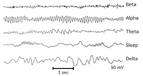
Fig.1. EEG Frequency Band [13]

The position of the electrodes during EEG measurement directly affects the amplitude, phase and frequency of the EEG signals. Suitable sites for electrodes placement are frontal, parietal, temporal or occipital brain lobes. The most preferred layout scheme is the 10-20 EEG electrode positioning system and is shown in Figure 2.

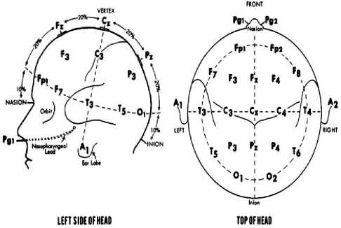
Fig.2. 10-20 EEG Electrode Positioning System [10]

As seen in Figure 2, the boundary for the electrode locations is the nose roots, nasion (above the nose), and innate bone in the occipital lobe. Thus, the surface of the skull is separated from the left and right segments. The ears are used as boundaries separating the skull surface from the front and the back. In this study, a 10-20 electrode positioning system is used for EEG measurements. The data was taken from three channels for two patients and obtained from five second epochs. For each patient, pre-seizure and non-seizure episodes were evaluated. Table 1 shows demographic information and number of samples of two patients from the Physio Net database [14].

Table 1. Demographic Information and Number of Samples

Patient’s Number	Age	Gender		Pre-Seizure	Non-Seizure
1	11	Female		80	192
8	2	Female		112	192

B. Creating the Database

In forming the database, firstly EEG signals obtained with surface electrodes are sampled at 256 Hz. A 10-20 electrode positioning system is used as the electrode system. The starting times and total seizure times of the data in the records are determined by the experts.

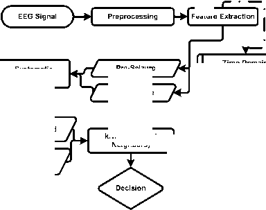
• III.    Recommended Method

As mentioned in the previous sections, the proposed method basically has a signal flow diagram consisting of the feature extraction, selection and classification steps starting with pre-processing of EEG signals. The flow diagram of proposed method is shown in Figure 3.

Feature

Decision

Systematic Sampling

Eta Correlation

Time Domain

Pre-Seizure

Non-Seizure

UnCorrelated

kNN (k-Nearest Neighbors)

» Mean

» Standard Deviation

» Variance

» Mode

» Hjorth Activity

» Hjorth Mobility

» Hjorth Complexity

» Renyi Entropy

» Entropy

» Maximum

» Minimum

» Zero Crossing Rate

» Burg Method

» Total Power

Frequency Domain

» Delta Band Power

» Theta Band Power

» Alpha Band Power

» Beta Band Power

Fig.3. Flow diagram of the recommended method

• A.    Pre-processing

Data from non-seizure and pre-seizure records are divided into five-second epochs. In our study, operations are performed for two epilepsy patients. Pre-seizure data is obtained for an 80-second time slot before the onset of seizure.

As a result, a total of 576 episodes of five-second epochs are collected from each patient, 192 of which were labeled "Pre-seizure" and 384 were "Seizure-free". EEG measurements were examined for three different channels.

• B.    Feature Extraction

In the majority of practical applications, the original signal is transformed into a new variable space with the aim of reaching the goal of the method more easily, that is, subjected to a preprocess. This preprocessing is often referred as feature extraction. A feature extraction from a signal is determining the distinguishing basic characteristics or attributes of the signal. Some properties are directly recognizable, while others are obtained after applying special operations on the job and are called artificial properties. In the feature extraction step, the goal is to define properties that enable fast calculation, distinguishing information, and accurate classification. The attention should be paid to the information that is emitted when the feature extraction operation is performed. If this information is important for the solution of the problem, the accuracy of the whole system is affected.

In the feature extraction step of the proposed method, distinguishing features defined in time and frequency domain are determined. These properties are shown in Table 2. The name of each feature, domain information and the formulations are also given in the Table 2.

When the values given in Table 2 are calculated in the extraction step, it is seen that the values contain diversity in pre-seizure period and normal seizure period.

• C.    Feature Selection with Eta Correlation Coefficient

Correlation is a commonly used definition for the purpose of measuring the relationship between two variables or distributions. In order to clarify the relation amount of correlation with another expression, correlation coefficient which can be valued in [-1,1] range is defined instead of correlation. Here, -1 means that there is a complete inverse relationship between two variables or distributions, and +1 means that there is a complete linear relationship between two variables or distributions and 0 means there is no relation. The Eta correlation is defined as the point biserial correlation coefficient in case of one of the variables to be examined is the two-categorical qualitative, the other is the continuous numeric data type, and is represented by r in Equation (1) as follows:

Table 2. Characteristics of EEG signals, description and formulas

EEG Feature Number Feature Explanation Formula 1 Mean Time N M = — Ух„ N Z n 2 Standard Deviation Time N Z (X n - M)2 SD = 1 -n=1----------- V   N-1 3 Variance Time v = SD2 4 Hjorth Activity Time HA = ct02 To : variance of signal 5 Hjhort Mobility Time HM = t / t0 T variance of 1.th derivate of signal 6 Hjhort Complexity Time HC = ^(T2/ T1)2 - (T1/ T0)2 T :variance of 2.th derivate of signal 7 Delta Band Power (0.5-2 Hz) Frequency N p=-ЁК-21 N2? i 8 Delta Band Power (2-4 Hz) Frequency 9 Theta Band Power Frequency 10 Alfa Band Power Frequency 11 Beta Band Power Frequency 12-19 Autoregressive Model Time ACR =-^z ap (i) x(n - i) + ^(n) i=1 a : AR parameters 20 Total power Time N P = -Z|x,2 | N ^f i 21 Maximum Time max V = max [ Xn ] 22 Minimum Time min V = min [ Xn ] 23 Mode Time M= the most frequently occurring value in vector X. 24 Entropy Time E = -Z P(Xi^logL P(Xi) 25 Renyi Entropy Time RE = T^ln Z xq q = 2 1 - q    i 26 Zero Crossing Rate Time ZCR = ^ |sgn [x(n)]- sgn [x(n- 1)] 1 rpb

Y Y

S y

P ₀ P ₁

S y = J < Z ^Y ’ - < Z ^Y > 2 / n )/n

Y and Y are mean values of pre-seizure and nonseizure period data respectively while P and P are the ratio of the number of samples to the total samples of preseizure and non-seizure period respectively. S_Y is the standard deviation of all observations and can be calculated using Equation 2.

In Equation 2, Y = [YY2 ]T is the observation vector [16]. In the study conducted, 26 feature are obtained for each of the 80 epochs of the pre-seizure and non-seizure normal period during the feature extraction step. Y1 and Y2 are both matrixes with the dimensions of 80x26. In this case, the correlation between the matrix columns representing the characteristics of each epoch is calculated while the Eta correlation is calculated. In conclusion, 26 Eta correlation values are obtained from the data of each patient. Absolute values are taken after Eta correlation values are calculated. Figure 4 illustrates how to perform the feature selection step.

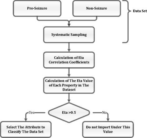
Fig.4. Eta Correlation Feature Selection Steps

As seen in Figure 4, first step is to systematic sampling by taking signals from epileptic seizure and non- seizure period. As a result of systematic sampling, there are 80 pieces of data consisting of five seconds epochs for each patient. Following to this step, feature subtraction is applied for each data. At the end of this step, a matrix of size 80x26 is obtained for the two patients mentioned in Table 1. Eta Correlation coefficients are calculated using Equations (1) and (2) so that the feature selection process can be performed. The features which have Eta correlation values greater than 0.5 are selected and other features are subtracted from the feature vector. The feature selection step reduces the size of the feature vector so that the computational load is reduced. It is also expected that the accuracy of the method obtained with the feature selection step will be improved.

• D.    k-Nearest Neighbor Based Classification

kNN is a simple and widely used classifier in signal processing applications. This algorithm is a non-linear and heuristic algorithm that basically compares the existing data with a new sample and decides which class to include. The main idea is that: the closest points in the feature space should have similar characteristics (17). In the decision phase, a new sample is assigned to the class by the majority vote of its k neighbors. k is chosen according to the distribution of feature space [18]. In the study, two groups are formed with and without Eta correlation. These two test groups are classified by classifier of kNN and the reality of the results is analyzed.

• E.    Statistical analysis

The characteristics of the EEG signal are not normally distributed. For this reason, the Mann-Whitney U test, which is a nonparametric counterpart of two independent sample tests, was used to compare pre- and non-seizure epilepsy data with each other. The p -value obtained as a test result gives a statistical probability value. If p <0.05, there is a significant difference between the two groups. If p >0.05, there is no significant difference between the two groups. The Mann-Whitney U test results obtained for the feature vector are given in Table 3.

• IV.    Performance Evaluation

The aim of this section is to evaluate the performance of the proposed study. For this purpose, the results of statistical analysis are given at first. Then, the classification results are discussed in details.

Since the characteristics of EEG signals are not normally distributed, the minimum, maximum and average values, standard deviation, upper and lower bounds of 95% confidence interval, Eta and Eta square values are calculated in the study. The p value which is utilized for feature selection is calculated by the Mann-Whitney U test. These values are illustrated in Table 3. In Table 3, p values lower than 0.05 are significant.

Briefly describing the features in Table 3, for example, in the first characteristic, the minimum value of the distribution before the seizure is -10.247, the maximum value is 20.928, the average value is 0.370, and the standard deviation is 3.274 The standard deviation indicates the range of values around the average of the data set. The lower and upper limits of the 95% confidence interval are -0.242 and 0.983, respectively. R Eta value is 0.032 and Eta square value is 0.001. This feature is not included in the new feature vector because the Eta value is smaller than 0.5 in feature selection phase. The p value is 0.822 and is meaningless for classifier performance. As a result, eight features were selected by considering the Eta value of the table. It can now be safely said that the selected instances are distinctive for the seizure and non-seizure period.

Table 3. Mann-Whitney U Test Results (There are nine features in the first two parts and eight features in the last part)

Feature No			1	2	3	4*	5*	6*	7	8	9	10*	11	12*	13
h о z	Min		-10.247	19.122	365.646	0.004	0.696	0.065	47.396	23.427	24.729	10.238	5.119	-1.961	0.049
	Max		20.928	118.908	14139.01	0.089	1.304	0.298	3568.04	868.316	460.084	116.951	85.486	-1.063	1.417
	Mean		0.37	41.565	2099.89	0.032	0.948	0.169	586.505	163.829	135.61	47.723	19.121	-1.723	1.11
	Std		3.274	19.381	2179.20	0.022	0.122	0.062	688.006	156.561	94.308	22.379	12.537	0.125	0.219
	%95 CI	LB	-0.243	37.936	1691.85	0.028	0.925	0.157	457.682	134.515	117.952	43.532	16.773	-1.747	1.069
		UB	0.983	45.194	2507.92	0.036	0.971	0.18	715.327	193.144	153.268	51.913	21.468	-1.7	1.151
h V	Min		-18.444	16.977	288.211	0.008	1.085	0.087	11.17	19.206	17.853	9.22	9.333	-1.541	0.589
	Max		19.207	113.912	12975.96	0.997	1.349	0.999	5081.05	930.496	398.712	58.991	34.454	-0.969	1.258
	Mean		0.169	30.741	1336.20	0.387	1.255	0.574	348.466	107.055	76.299	20.443	19.949	-1.208	0.966
	Std		2.859	19.868	2306.81	0.267	0.065	0.24	847.562	180.896	77.308	7.071	5.699	0.139	0.119
	%95 CI	LB	-0.366	27.01	904.272	0.337	1.243	0.529	189.768	73.184	61.824	19.119	18.882	-1.234	0.943
		UB	0.704	34.461	1768.13	0.437	1.267	0.619	507.164	140.926	90.774	21.767	21.016	-1.182	0.988
R(Eta)			0.033	0.267	0.168	0.685	0.845	0.758	0.153	0.166	0.327	0.637	0.043	0.891	0.38
R2			0.001	0.071	0.028	0.469	0.714	0.574	0.023	0.028	0.107	0.405	0.002	0.793	0.145
p			0.822	0	0	0	0	0	0	0	0	0	0.002	0	0

Feature No			14	15*	16*	17	18	19	20	21	22	23	24	25	26*
1 о z	Min		-1.292	0.389	-0.508	-0.457	-0.014	-0.272	365.379	57.241	-332.7	-98.266	1.012	-16.741	0.016
	Max		0.01	1.074	-0.047	0.04	0.599	0.221	14565.96	442.1	-53.333	48.645	1.259	-13.056	0.1
	Mean		-0.814	0.704	-0.223	-0.267	0.307	-0.07	2109.01	124.727	-125.108	-2.965	1.142	-14.429	0.055
	Std		0.236	0.145	0.102	0.137	0.139	0.077	2205.05	64.292	57.151	16.68	0.055	0.831	0.02
	%95 CI	LB	-0.858	0.677	-0.242	-0.292	0.281	-0.085	1696.14	112.689	-135.808	-6.089	1.132	-14.585	0.051
		UB	-0.769	0.732	-0.204	-0.241	0.333	-0.056	2521.88	136.765	-114.407	0.158	1.153	-14.274	0.058
1 V	Min		-1.343	0.058	-0.23	-0.454	-0.04	-0.219	288.741	48.645	-540.95	-92.015	1.031	-16.625	0.026
	Max		-0.525	0.685	0.289	0.179	0.429	0.115	12972.70	342.47	-44.347	37.314	1.284	-12.82	0.35
	Mean		-0.96	0.386	-0.03	-0.198	0.184	-0.061	1343.29	94.683	-103.346	-1.622	1.176	-13.775	0.194
	Std		0.154	0.117	0.1	0.117	0.11	0.078	2317.68	49.055	67.778	13.823	0.052	0.851	0.083
	%95 CI	LB	-0.989	0.364	-0.049	-0.22	0.164	-0.075	909.324	85.498	-116.036	-4.21	1.166	-13.935	0.179
		UB	-0.931	0.408	-0.012	-0.176	0.205	-0.046	1777.25	103.869	-90.655	0.966	1.185	-13.616	0.21
R(Eta)			0.346	0.771	0.692	0.262	0.442	0.063	0.168	0.255	0.172	0.044	0.296	0.364	0.759
R2			0.119	0.594	0.478	0.069	0.196	0.004	0.028	0.065	0.03	0.002	0.088	0.132	0.575
p			0	0	0	0	0	0.203	0	0	0	0.429	0	0	0

In order to evaluate the performance of the presented method, some of the commonly used criteria are defined in this section. These criteria are accuracy, error rate, precision, sensitivity and F-measure. To calculate these measures confusion matrix is widely used in the literature. The confusion matrix demonstrates the relationship between actual results and test results. In other words, this matrix represents how close or far the test results are to the truth. The structure of the confusion matrix is given in Table 4.

Table 4. Structure of the confusion matrix

		Actual Results
		0 (Pre-Seizure)	1 (Post-Seizure)
> и z	0 (PreSeizure)	TP(True Positive)	FP(False Positive)
	1 (PostSeizure)	FN(False Negative)	TN(True Negative)

Among performance evaluation criteria, accuracy is one of the most popular and simple criteria. This criterion is the ratio of the number of correctly classified samples ( TP + TN ) to the total number of samples ( TP + TN + FP + FN ) . The error rate is defined as the value that completes the accuracy ratio. Precision is the ratio of the number of samples that are estimated to be class 1 and the number of samples that are really 1, ie True Positive ( TP ) , to the total number of samples ( TP + FP ) estimated as class 1. The ratio of correctly classified positive sample ( TP ) to sample number ( TP + FN ) is called sensitivity. The F-criterion is the harmonic mean of the precision and sensitivity. Precision and sensitivity criteria alone may not be enough to result in a meaningful comparison. Evaluating both criteria together gives more accurate results [19]. For this reason,

Table 5. Evaluation criteria and formulas

Evaluation	Formula
Accuracy	TP + TN x 100 TP + TN + FN + TN
Error rate	FP + FN TP + TN + FN + TN
Precision	TP TP + FP
Sensitivity	TP TP + FN
F-measure	2 SA S + A

* TP=True Positive, TN=True Negative, FP=False Negative, FN=False Negative, S=Sensitivity and A=Accuracy the F-criterion is used as a performance criterion. Mathematical representations of these measures described in Table 5 are given.

• V.    Results

In our study, we first performed the pre-processing step of epilepsy patients' data. Then, 26 characteristic features of the EEG signals are obtained. Two test clusters are constituted from the specified properties. The results of statistical analysis are given at first. Then, the classification results are discussed in details.

Since the characteristics of EEG signals are not normally distributed, the minimum, maximum and average values of signal, standard deviation, upper and lower bounds of 95% confidence interval, Eta and Eta square values are calculated in the study. The p value which is utilized for feature selection is calculated by the Mann-Whitney U test. These values are illustrated in Table 3. In Table 3, p values lower than 0.05 are significant. The Eta correlation is used for the feature selection phase. The features which have p values lower than or equal to 0.05 remained in the feature vector. On the other hand the features which have p values higher than 0.05 are eliminated. At the last stage, the properties obtained from the test clusters have been subjected to classification by the classifier of kNN. The classification results are given in Table 6.

Table 6 shows the kNN classification results of Eta-correlated and uncorrelated features. The effect of Eta correlation on training and test data is clearly visible on the table. For example, the uncorrelated accuracy results for training and test data in the second channel are [91.071%, 86.607%] while the Eta-correlated accuracy results for the training and test data are [91.964%, 92.857%]. That is, the Eta correlation increases the accuracy rate. Increasing the accuracy rate reduces the error rate, increases the precision and sensitivity of the system. Since the F-criterion is the harmonic mean of the precision and sensitivity, the F-measure is also increased.

• VI.    Discussions

In this study, we aimed to use EEG signals to automatically detect pre-epileptic periods of the epilepsy patients with machine learning techniques. EEG data for two epileptic patients are used in the proposed study. The EEG data is passed through the preprocessing stage and then subjected to feature extraction in time and frequency space. In the feature extraction step 26 features are obtained to determine the seizure time. When the feature vector is analyzed, it is seen that the characteristics of the pre-seizure and non-seizure periods are unevenly distributed. A systematic sampling method has been applied for this imbalance. For the balanced data, two test clusters with and without Eta correlation are established. Finally, the classification process is performed applying the kNN method. The results are evaluated in terms of

Eta-correlated and uncorrelated accuracy, error rate,      Various simulations have been conducted with the aim precision, sensitivity and F-criterion for each channel.        of evaluating the performance of the presented method.

Simulation results are given in Tables 3 and 6.

Table 6. Training and Test Results of KNN Classifier

Training and Test Results

	Uncorrelated		Eta Cor.		Uncorrelated		Eta Cor.		Uncorrelated		Eta Cor.
	1.Channel		1.Channel		2.Channel		2. Channel		3. Channel		3. Channel
	Training	Test	Training	Test	Training	Test	Training	Test	Training	Test	Training	Test
Accuracy	83.036	78.571	88.393	85.714	91.071	86.607	91.964	92.857	91.071	82.143	87.5	82.143
Error rate	0.17	0.214	0.116	0.143	0.089	0.134	0.08	0.071	0.089	0.179	0.125	0.179
Precision	0.849	0.857	0.922	0.75	0.859	0.911	0.898	0.929	0.897	0.839	0.828	0.946
Sensitivity	0.804	0.75	0.839	0.955	0.982	0.836	0.946	0.929	0.929	0.81	0.946	0.757
F-measure	0.826	0.8	0.879	0.84	0.917	0.872	0.922	0.929	0.912	0.825	0.883	0.841

As can be seen from Table 3, the minimum and maximum values of the extracted properties show significant differences for the pre-seizure and normal data groups. Similarly, the minimum and maximum values of the 95% confidence interval for features show significant differences between the groups. For example, in the case of epilepsy pre-seizure, the interval of 95% confidence interval is [37.936, 45.193] while in the absence of seizure this interval is [27.020, 34.460].

The average values given for the properties can be considered as the central point of the distribution for the groups. When the average values of the groups are examined, it is seen that the center is far away from each other. For example, the average pre-seizure value for feature 10 is 47.722, while the mean value for seizure-free turnaround is 20.442. On the other hand, the standard deviation indicates the distribution of the data group around the center. Again, for the feature 10, the standard deviation before the seizure is 22.378 while the value at the seizure is 7.070.Compared to the standard deviation values, it can be said that the pre-seizure moment is more scattered.

Now, we can compare our study with an existing method in the literature. In [3], authors utilized EEG signals to predict the epilepsy seizure by using kNN. Their accuracy, precision and sensitivity results are 94.80%, 93%, 96.50%, respectively. As given in Table 6, these measured obtained by our study is better than that of [3]. In addition, in [3] authors performed SVM and MLPNN classifiers for the same purpose and they achieve increased performance with these classifiers. So, in our following study we will compare classifying results of kNN, SVM and MLPNN methods on a wider database. To improve the performance of compared classifiers we will try to derive new features in the transform domain especially in the wavelet domain. Furthermore, instead of using synthetic data we will take real time EEG data from the epilepsy patients by means of working with a specialist.