Automated recursive separable algorithm for medical image processing

Digital image processing is one of the important areas of development of computer technologies used in modern telemedicine. Particular attention is paid to improving the quality of images, restoring damaged images. Image processing technology has a number of advantages, such as flexibility, adaptability, data storage and communicativeness - it has many rules for synchronous image processing. Two-dimensional and three-dimensional images can be processed in several dimensions (image processing methods were founded in the 1960s), these methods have been used in various fields, such as medicine, space, clinical research, art, etc. [1].

Medical imaging and diagnostic techniques have developed rapidly in recent decades and have become a very important part of disease diagnosis. Digital medical images (DMI) play an important role in transmitting information about the heart, brain, nerves, etc. to obtain an internal view of the human body. Numerous mathematical applications can be applied to medical images to conclude whether healthy tissue is infected or not. However, the loss of any specific area during medical imaging can lead to disaster such as death. The main challenge in the process of medical imaging is to obtain an image without losing any significant information [2].

It should be noted that in a number of areas of DMI research, the conducted scientific research on the automation of image processing and analysis yield worse results compared to manual image analysis by specialists [3]. Existing software products for DMI processing yield good results, but they are usually foreign products with closed specialized software built into the analysis device and supplied with it. This foreign equipment is expensive. The development of domestic software for analyzing and improving the quality of visual information is an urgent task, the solution of which will allow processing large volumes of information obtained in the field of telemedicine [4].

In the modern world, many scientists are developing automated algorithms for processing and analyzing digital images that can increase human productivity. The work [5] presents Mitometer, an algorithm for fast, unbiased, and automated segmentation and tracking of mitochondria in live-cell two-dimensional and three-dimensional time-lapse images.

A number of modern studies such as an artificial intelligence-based algorithm for automated diabetic retinopathy screening [6], methods for visual object recognition for automated digital modeling of existing buildings [7], a study on the impact of a real-time automatic quality control system on the detection of colorectal polyps and adenomas [8], an approach and dataset for describing document feature points using a small convolutional neural network [9], a method for segmenting breast cancer boundaries and pectoral muscles in mammograms using threshold-based and fully automated trainable approaches [10], a deep learning method for automatic medical image segmentation requiring minimal annotations [11], and an artificial bee colony algorithm and its application in medical image processing [12] present various methods for automating DMI processing algorithms and their application for various telemedicine tasks. In addition to the automation of image processing algorithms, algorithms for automated assessment of the quality of processed images are also being actively developed; for example, the work [13] presents an automated visual assessment.

• 1.    Develop an automated algorithm;

• 2.    Implement an application for using the developed algorithm;

• 3.    Perform testing of the implemented algorithm.

1.    Digital filter

The automated algorithm is implemented on the basis of a two-dimensional digital Laplacian Filter “double pyramid” (LDP) [14 – 15].

The two-dimensional digital LDP filter in the implementation of the size 7 x 7 (Fig. 1) is a filter in the center of which there is a positive aperture of 3 x 3 elements.

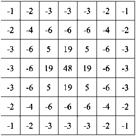
Fig. 1. Three-dimensional view of the LDP filter aperture

The structural diagram demonstrating the operating principle of the filter used is shown in Fig. 2.

The filter operates according to the following principle. In the second branch, a mask is formed, with a given dimension of the corresponding coefficients of the frame and line recirculators. Recirculators use the recursion property to search for each result obtained after the first sample is formed, which allows to reduce the image processing time. It is the main one and is fed to the adder with a negative sign. In the first branch, a second mask is formed with the same dimension as the internal mask from the lower branch. In this case, it has a certain coefficient X, with which the convolution by the line and frame recirculators will occur. It is fed to the adder with a positive sign.

In the third branch, an additional mask is formed, which performs a similar function as the upper branch of the original filter. This branch has a coefficient A 2 , which participates in increasing the central element. This branch is also fed to the adder with a positive sign. As a result, the matrix of the digital filter is formed.

2.    Automated processing algorithm

The filter algorithm consists of the following steps:

• 1.    Entering basic parameters. It is necessary to enter the input data: h – mask size value (odd); X – image to be processed; A 1 – central aperture lift coefficient; A 2 – central element magnification coefficient.

• 2.    Determining the recirculator values for convolution of the processed image into the original matrix.

• 3.    Calculating the main filter matrix, which consists of calculating the coefficients of two frame and two row recirculators.

• 4.    Calculating the shift coefficients of the additional (internal) mask and calculating the size of this internal mask.

• 5.    Calculating the coefficients of the frame and row recirculators for the second (additional) matrix.

• 6.    Calculating the coefficient A 1 , which is the main coefficient for convolution.

• 7.    Convolution of the original image with these recirculators, taking into account the coefficient A 1 , the central aperture lift regulator.

• 8.    Formation of an additional matrix.

• 9.    Surrounding the resulting matrix with zeros to the size of the main one.

• 10.    Formation of a third matrix to implement the lifting of the central element.

• 11.    Final calculations.

For the software implementation of the constructed automated recursive-separable algorithm for processing medical images, the Python programming language was chosen, where the algorithm of all processes occurring in the filter is written in the form of code. Fig. 3 shows a block diagram of the automated algorithm for processing digital medical images.

The initial digital image is fed to the input of the algorithm, the algorithm takes one color channel of the image and starts working. The mask size is entered from the keyboard, the entered value must be odd. To enter the parameters A 1 and A 2 , a nested loop was created that automatically iterates over the values in the range specified by the user. After entering the initial parameters, the image is processed by the algorithms described in the previous paragraph. When the image processing is finished, the image quality assessments such as the mean square error MSE, the structural similarity index SSIM and the peak signal-to-noise ratio PSNR are calculated.

MSE is the most common metric, and the closer its value to zero, the better. It is also called the deviation of the evaluator, which is the original image. The error is the difference between the estimated result and the evaluator [16]. PSNR is used to quantitatively evaluate the effectiveness of different noise reduction methods. It is a measure of the peak error, used as a measure of reconstruction of lossy compression codes. The signal is the original image, and the noise is the introduced compression. The higher the value of the ratio, the more the reconstructed image is similar to the original [17].

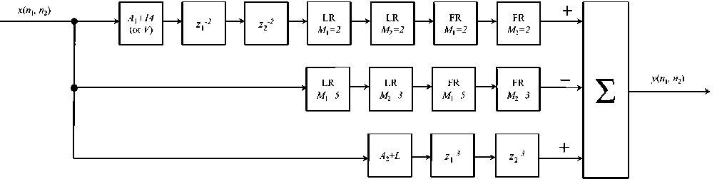
Fig. 2. Structural diagram of the LDP filter:

x(n 1 ,n 2 ) – input data; 14 (V) – coefficient for additional mask convolution; z 1^-2 and z 2^-2 – delay by two elements; LR - line recirculator, FR -frame recirculator; M 1 – line direction, M 2 – frame direction; z 1^-3 – delay by three elements; A 1 – coefficient of rise of the central aperture;

A 2 – coefficient of increase of the central element; y(n 1 ,n 2 ) – output data; L - coefficient of the complementary matrix

The structural similarity index of image (SSIM) is a relatively new method for measuring image similarity, used in areas ranging from image restoration/compression to object recognition [18].

Image processing ends with the formation of the final matrix with normalization of the image brightness, this matrix is larger in size than the matrix of the original image, therefore, to calculate image quality estimates, it is first necessary to crop the matrix to the desired size, thus obtaining a mask. To calculate the peak signal-to-noise ratio, it is necessary to know the root-mean-square error, therefore this parameter is initially calculated. After the MSE value is known, the PSNR is calculated.

The PSNR and MSE parameters provide a general integral assessment of image quality. It is believed that good image quality is ensured at PSNR > 40 dB and SSIM > 0.98 [19]. Accordingly, after calculating the image quality estimates, the obtained values are compared with the values at which the image is considered to be of good quality. If the value of the processed image satisfies the values of a good quality image, the image is saved with the parameters A 1 and A 2 indicated, the values of the processed image are output, and a message is output to the console stating that the image has been saved.

The original image (x(n1, n2)) is processed by the line (LR) and frame (FR) recirculators using the values obtained during the calculations. The size of the first line and frame recirculator is denoted by M1, and the size of the second line and frame recirculator is denoted by M2. The calculation process is performed as follows: in the calculation algorithm, the minimum value of the recirculator is specified, for the LDP filter it is equal to 3 (t1 =3), and then the difference between the user-entered value of the filter aperture size (h) and the coefficient t1 is found. The result is divided by 2 (k =(h – t1) /2). Then the obtained value is added to the coefficient t1, hus the value of the coefficients of the first recirculators is calculated (M1 = t1+k). The value of the coefficient of the second recirculators (M2) s calculated based on M1, and the coefficient 2 is subtracted from it (M2 = M1 – 2).

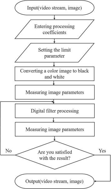
Fig. 3. Block diagram of the automated recursive-separable algorithm

Next, the algorithm is launched, constructing a matrix of values, after processing the original image by the recirculator LR (M1). To begin with, the recirculator Y1, itself is designated, it takes the size of one row and the number of columns equal to M1, which was calculated earlier. Then the algorithm determines the values of the number of columns and rows in the original image X, as well as the number of columns in the recirculator, and writes them as i1, j1 and i2.

Next, the algorithm builds the matrix X 1 from the original image and supplements it with zeros on the right to the final size. Then it determines the coefficients k and m . They are necessary for building the basis for recording the future result, the zero matrix y 1 .

When all the initial data is ready, the code starts a two-level cycle. First, it selects a row of the y 1 , matrix, then a column, and fills the column with the necessary values. So, in the first column there will be a value equal to the value of the same element in the X 1 matrix. In the second column, the value of the element in the X 1 matrix will also be taken into account, and in any case, whether there is a certain number or zero, the algorithm will accept it and add the previous element of the y 1 matrix to it. Such operations will be performed until it passes the middle and reaches a certain element, when the value begins to change. Then it will set values with the elements equal to the value of the X 1 element plus the values of the previous element and minus the value of the X 1 element, which is in the first column.

The result is a matrix ( y 1 ), where the number of rows will be equal to j 1 x i 1 + i 2 – 1.

The same thing happens with the second row recirculator. The only difference is that instead of the original image, the final matrix ( y 1 ), obtained after the first recirculator, is taken (Fig. 4).

for к in range (0, jl):

for m in range (0, il+(i2-l)):

if m==0:

y2[k,m]=X2[kfm]

if m>0 and m

y2[k,m]=X2[kfm]+y2[k,m-l] if m-i2>=0:

y2[k,m]=X2[k,m]-X2[k,m-i2]+y2[k,m-l]

• Fig. 4.    Fragment of the code for the operation of the second line recirculator

Similar work is performed by frame recirculators (FR). Similar to the second row recirculator, the matrix obtained as a result of work at the previous stage (y2) is taken as a basis. The matrix is surrounded by zeros from above and below to the final size, and in the cycle itself the work is performed by columns, and not by rows, as before. That is, first a column is selected, filled with elements, and only after that it moves on to another column.

The second frame recirculator operates in the same way. However, this time the final matrix obtained after the first frame recirculator (y3), respectively, and after two row recirculators, i.e. the result of all previous convolutions, is taken as the initial matrix and the basis for convolution. As a result, the matrix of the result of all operations in the filter branch (y4) is obtained.

The process of calculating the central mask shift factor is based on the use of the h value, i.e. the mask aperture size.

The aperture size value is increased by one (h + 1), thereby bringing it to parity. Then a check is made, i.e. in this case, the value is filtered for the possibility of dividing by 4. If the value is divisible by 4, it is divided, and as a result, the shift factor is obtained for the elements z1^{– n} and z2^{– n}.

The process of calculating the recirculator coefficient for the central mask of a filter with an aperture of 7x7 elements is based on the use of the h value. The aperture size value is increased by one (h + 1), thereby bringing it to parity. Then a check is made, that is, in this case, the value is filtered for the possibility of dividing by 4. If the value is divisible by 4, then it is divided, and as a result, the coefficient M1 = M2, is obtained, for LR and FR in the first branch of the filter.

Next, the convolution coefficient V is calculated (in the special case of 7x7 elements, it is equal to 14). It should be calculated based on the value required to achieve the goal at which the sum of the internal and external elements of the final matrix will be equal to zero A fragment with the calculation of the convolution coefficient is shown in the Fig. 5.

S0=(tll*t22)*(tll*t22)

P=(t33*t33)*(t33*t33)

A=S0//P

Aground(A)

• Fig. 5.    Code snippet with calculation of convolution coefficient

3.    Implementation of an application for using an automated algorithm

The coefficient for convolution is calculated according to the following principle. First, the sum of the elements of the main matrix is found. It is the multiplication of the coefficients of the recirculators. Thus, the summation is not of the matrix that was obtained during processing of the received image, but of the matrix calculation when feeding a unit as the original image.

Since the final summation must be carried out with matrices of the same dimensions, the resulting matrix is surrounded by zeros up to the size of the main one.

The resulting matrices, when summed, will not give a sum of elements equal to zero, therefore a third matrix is formed.

The formation of this matrix occurs according to the following principle. First, the coefficient L is found. It is based on finding the missing value, therefore, first, the sum of the elements of the additional matrix is calculated. The found coefficient V is also taken into account, it is multiplied by the sum of the elements when convolving the unit with an additional mask, that is, as a result, the sum of the matrix elements is obtained when convolving the coefficient V instead of the unit.

Then the missing value is found. For this purpose, the code refers to the value of the sum of the elements of the first matrix when convolving one. The found sum of the elements of the additional matrix is subtracted from it, and as a result, the missing value is obtained. It is the coefficient L. To begin with, the original image is multiplied by the sum A2+V, then the process of adjusting the obtained element to the size of the main matrix occurs. A zero matrix is constructed with the same size as the main one, which will serve as the basis. And then the shift coefficient is determined by adding one to the second value of the recirculators of the main matrix. And ultimately, a zero matrix is formed, in the middle of which the central element or matrix is placed.

The final stage of the filter operation is the summation of all the obtained masks. However, when the central matrix and the central element are raised, the image brightness values are violated; in order to normalize it, the final sum of the matrices is divided by the sum of the elements that were added using A1 and A2. The resulting matrix will be the result of the filter operation [20].

To use the automated recursive separable algorithm for processing medical images, a software module [21] was implemented using QtDesigner and PySide6.

The software module consists of three areas for inputting data, such as the mask size h, the coefficient for lifting A1 and the coefficient for increasing the central element A2, two areas for displaying the image, the original and processed, seven buttons, such as input, output and saving the image, checking the image quality condition, three buttons for calculating the MSE, PSNR and SSIM parameters.

To operate the buttons, the previously developed and described algorithm was divided into functions. A certain function is responsible for the operation of a certain button.

A separate function was written for the windows that appear on the user’s screen, which report the successful loading, output and saving of the image, display a window with the results of calculating the MSE, PSNR and SSIM parameters, and also display the result of checking the image quality conditions (Fig. 6).

The function for the "Insert image" (кнопка «Вставить изображение») button specifies the dimensions of the window into which the image will be inserted, as well as messages that will appear in the event of a successful or unsuccessful attempt to load the image.

The function for the "Calculate MSE" (кнопка «Рассчитать MSE») button specifies the lines for displaying messages on the user's screen, and also specifies all the necessary parameters for calculating the value.

The function for the "Calculate PSNR" button (кнопка «Рассчитать PSNR») specifies the lines with messages for windows with notifications and specifies the necessary parameters. To calculate PSNR, the necessary parameter is MSE; if it is not calculated, an error will occur.

In the function for the "Calculate SSIM" button (кнопка «Рассчитать SSIM»), the required parameter for calculation is the resulting matrix obtained as a result of the algorithm. If the matrix is not calculated, an error occurs.

The function for the "Output image" button (кнопка «Вывести изображение») is similar to the image input function. It also specifies the size of the window in which the processed image will be output.

The function for the "Condition check" button (кнопка «Проверка условия») requires the previously calculated PSNR and SSIM values, otherwise the user will see an error message.

• ■¹ MainWindow                                                                                  — О X

Плодное изображение                                   Готооое изображение

Вставить изображение                                   Вывести изображение

Введите размер маски

Рассчитать MSt

Введите коэффициент дал подъема                                             Рассчитать PSNR

______________________________________________________________ Рассчитать SSIM

Введите увеличение центрального элемента                                    Промеры условия j                Сохранить изображение

Fig. 6. Appearance of the software module

The function for the "Save image" button (кнопка «Сохранить изображение») allows you to save an image with a unique number using the coefficient values entered at the beginning of the algorithm.

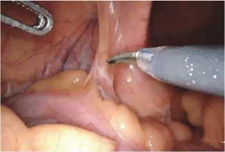
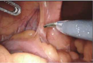
4.    Testing the automated algorithm

The performance test of the developed and implemented automated algorithm will consist of assessing its impact on a number of parameters.

As part of the experimental study, the desired parameters of the PSNR and SSIM metrics will be set, which the algorithm must achieve during its operation, and a fixed value of the filtering coefficient A1 = 1. As a result of the algorithm's operation, the operating time will be obtained, during which it was possible to achieve the specified values of the PSNR and SSIM metrics, as well as the value of the additional filtering coefficient A2.

The study will be conducted on a computing platform with the following characteristics: processor – Intel(R) Pentium(R) CPU 5405U @ 2.30GHz; RAM – 4 GB; system type – 64-bit.

In the original image, the values of the parameters were as follows: PSNR= 13.994; SSIM=0.452.

Fig. 7 Shows a test image that will be used in the experiment.

The parameter values were obtained using the equations below. All equations were written in the code and calculated sequentially.

The mean square error is measured using Eq. (1):

(M. N)                             2

^{MSE =}U_XN £ [ Ilj I2 (i- ¹ ^ '       (‘)

where M x N - image size, 11 (i, j) - original image, 12 (i, j) - processed image.

Fig. 7. Test image

The peak signal-to-noise ratio is calculated using the following Eq. (2):

PSNR = 10log

I²

MSE

where I – the maximum value of an image pixel. If the input image has an eight-bit integer data type, this value will be 255.

The most common equation for measuring SSIM between x and y vectors is:

SSIM(x,y) = [l(x, y)]“ [c(x, y)]₽ [s (x,y)]7,(3)

where l – comparison of luminance signals (Eq. 4), c – comparison of contrast signals (Eq. 5), s – structural correlation of signals (Eq. 6).

l (x, y) = (2цxЦy + ci) / (Цx2 +Цy2 + ci),(4)

c(x,y) = (2oxоy + c2)/(ox2 + oy2 + c2),(5)

^ xy⁺c3

s (x, y ) = —----, о xy + c3

where ц_x, ц_y - average values of x and y, о_x2, о_y²- variance of x and y, c₁ , c₂ , c₃ – constant values for cases where σ and μ are too small.

Substituting all the data we obtain the final result.

The structural similarity index is calculated using Eq. (7):

_{SSIM ( x} y₎=    ^{( 2Ц}x^Цy⁺ci ^{)( 20}xy⁺c 2 ⁾

’     (ц x² +Ц y² + ci )(o x² +O y² + c 2 )

In the experiment, different levels of PSNR and SSIM metrics were set, with a fixed value of the filter coefficient A1 = 1. After that, the automated recursive separable algorithm was launched, within the framework of which it performed a step-by-step enumeration of the filter coefficient A2 and an assessment of the specified parameters. In cases where it was not possible to achieve the specified values of the PSNR and SSIM metrics, repeated processing was performed, but with a different value of the filter coefficient A2 until the desired result was achieved. As a result, information was also issued on the time spent on achieving the required result, these results are presented in Tab. 1.

Analyzing the obtained data, it can be seen that the higher the required values of the PSNR and SSIM parameters, the more time the algorithm needs to find the optimal coefficient. These results are logical and consistent.

Tab. 1. Test results of the automated recursive-separable algorithm

PSNR, dB	SSIM	Time hh:mm:ss	Coef. A2
15	0.35	00:00:26	A2 = 1
20	0.45	00:01:18	A2 = 5
25	0.55	00:04:22	A2 = 19
30	0.65	00:09:58	A2 = 47
35	0.75	00:20:27	A2 = 95
38	0.85	00:30:46	A2 = 141
40	0.98	01:58:55	A2 = 571

By analyzing the works [14– 15] it can be concluded that the algorithm’s performance has improved significantly, with the LDP filter showing a 6-fold increase in performance compared to the classical two-dimensional convolution.

In addition to the quantitative and time assessment, a visual assessment of the image quality was also carried out. Each image was saved when the parameters specified in the table were reached and did not acquire third-party artifacts. Fig. 8 shows a test image after processing by an automated algorithm.

Fig. 8. The result of the algorithm operation with PSNR ≥ 35 and SSIM ≥ 0.75

Conclusion

The developed automated algorithm of the LDP filter operation allows achieving the required results without user participation, in particular, increasing such image quality assessments as PSNR and SSIM. In the process of automating the algorithm, the ability to enumerate the lift coefficients and increase the central element until the value becomes equal to the parameters specified by the user was added to it.

As a result of testing the algorithm, the dependence of the growth of PSNR, SSIM, the algorithm operation time and the value of the filter coefficient was demonstrated. However, at this stage there is a significant drawback in the speed of the algorithm, with the initially low quality of the original images. In the framework of further work, it will be eliminated by optimizing the algorithms of the automated filter.

During the implementation of the automated algorithm, software was also developed that allows testing the algorithm and performing a visual assessment of the results obtained.