Automatic Removal of Artifacts from EEG Signal based on Spatially Constrained ICA using Daubechies Wavelet

Published Online July 2014 in MECS

Human brain possesses rich spatiotemporal subtleties Because of its complicated uncertain cautious nature. Electroencephalography (EEG) provides a direct determination of cortical behavior with millisecond temporal steadfastness when compared to supplementary techniques. Electroencephalogram (EEG) is multivariate time series data measured using multiple sensors positioned on scalp that imitates electrical potential produced by behaviors of brain and is a record of the electrical potentials created by the cerebral cortex nerve cells. There are two categories of EEG, which is based on location of the signal obtained in the head: scalp or intracranial. Scalp EEG as being the main focus of the research, uses small metal discs, also known as electrodes, which are kept on the scalp with good electrical and mechanical touch. Intracranial EEG is obtained by special electrodes placed in the brain during a surgery. The electrodes should be of minimum impedance, in order to record the exact voltage of the brain neuron. The variations among the voltage difference among electrodes are sensed and amplified before being transmitted to a computer program.

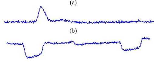
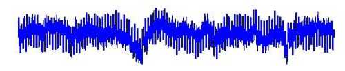
EEG data may be contaminated at many points during the recording and transmission process. Most of the artifacts are biologically generated by sources external to the brain. Improving technology can decrease externally generated artifacts, such as line noise, but biological artifacts signals must be removed after the recoding process. Figure 1 shows waveforms of some common EEG artifacts.

• •    Eye Blink artifacts: It is very common in EEG data, produces a high amplitude signal that can be many times greater than EEG signals into consideration. Because of its high amplitude an eye blink can corrupt data on all electrodes, even those which are at the back of the head. Eye artifacts are often measured more directly in the Electro-Oculogram (EOG), pairs of electrodes placed above and around the eyes. But unfortunately, these measurements are contaminated with EEG signals of interest and so simple subtraction is not a removal option even if an exact model of EOG diffusion across the scalp is available [2]

• •    Eye Movement : These artifacts are caused by the reorientation of the retinocorneal dipole [3]. The effect of this artifacts is sturdier than that of the eye blink artifacts. Eye blinks and movements often occur at close intervals.

• •    Line Noise: Strong signals from A/C power supplies can corrupt EEG data during transfer from the scalp electrodes to the recording device. Notch filters are often used to filter this artifacts containing lower frequency line noise and harmonics. Notch filtering at these frequencies can remove useful information. Line noise can disturb the data from some or all of the electrodes depending on the source of the problem.

• •    Muscle Activity : These artifacts are caused by activity in different muscle groups including neck and facial muscles. These signals have a wide frequency range and can be distributed across different sets of electrodes depending on the location of the source muscles.

• •    Pulse: When an electrode is placed on or near blood vessel, it causes pulse, or heartbeat, artifacts. The expansion and contraction of the vessel introduce voltage changes into the recordings. The artifacts signal has a frequency around 1.2Hz, but can vary with the state of the object. This artifacts can appear as a sharp spike or smooth wave [4].

дДд^^ '^ ^/ Xv^'%^

(e)

(f)

Fig.1 (a) Clean EEG, (b) Eye blink, (c) Eye movement, (d) 50 Hz, (e) Muscle activity, (f) Pulse.

EEG offers a continuous graphic display of varying voltage with time. However, the captured EEG [4-7] includes artifacts in the waveforms. Several researches have been organized to remove the artifacts in the EEG signal and various techniques are resulted due to this research.

The placement of the EEG electrodes on the scalp is standardized by the international 1020 system depicted in Figure 1.2. The electric field intensity of the EOG decreases with distance from the eyes when observing individual channels of the EEG from the frontal, central, and the parietal regions of the scalp [6].

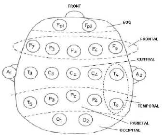
Fig.2. International 10-20 System for Electrode Placement (Top View)

This paper proposes a new technique for removing the artifacts [33, 34] from the EEG signal which uses kurtosis based on difference of Gaussian and SuperGaussian signal and Spatially-Constrained ICA (SCICA) [37, 38] and daubechies wavelet techniques. Threshold plays an important role in separating the artifacts from the non-artifact EEG [39]. Otsu’s Threshold is been adopted as the thresholding method in this paper. This method pre-assumes that EEG contains two classes namely, artifact and non artifact signal and further it calculates the optimum threshold separating those two classes.

II. Related Work

Artifacts noise in EEG are usually handled by dumping the affected segments of EEG. The humblest methodology is to discard a fixed length segment, perhaps one second, from the time an artifacts is detected. Discarding segments of EEG data with artifacts can

greatly decrease the amount of data available for analysis. EEG data collected from children is especially problematic in this respect [10]. The first attempts at removing artifacts focused on eye blinks. Regression using the EOG channel was attempted in the time and frequency domain [12, 11, 20, 24, and 25]. These methods all rely on a clean measure of the artifacts signal to be subtracted out. Since the EOG is contaminated with EEG signals, the regression of ocular artifacts has the undesired effect of removing EEG signals from the observations. A good review can be found in [8, 9]. Kenemans et al. [14] gave a general lagged regression model. Jung et al. [2] used this regression model for a baseline artifacts removal method. Multivariate statistical analysis techniques, such as principal component analysis, have been used to separate and remove noise signals from the brain activity of interest [5, 16, 2, 13, 17, 7, and 20]. Comparisons of artifacts removal using different transformations can be found in [26, 22]. Comparison of four methods for artifacts removal by artificially mixing an artifacts signal from one subject with a set of EEG signals from another subject is given in [22]. The artificial mixing matrices were chosen to approximate mixing in the scalp. Two independent component analysis methods studied in [6], were significantly better than principal component analysis and simple EOG subtraction. Performance was measured using the mean squared error between the true artifacts signal and the extracted artifacts signal. Significance was measured using an F-statistic and Tukey's studentized range test [22].

The common spatial patterns (CSP) technique, which requires the use of two data sets was used by Koles [15] to remove abnormal Components, It uses data from 80 patients. No quantitative evaluation was done on the removal but it was visually observed that the artifacts were extracted into a small number of components that would allow their removal. In online filtering systems, artifacts recognition is important for achieving their automatic removal. One approach to recognition of noise components is based on measuring structure in the signal. The fractal dimension and a metric based on autoregressive (AR) coefficients have been used for this purpose [7, 21].

Eye blinks and heart beats were found to have consistent fractal dimensions on the data studied [21]. Jung [2] suggests that the spectral structure might be distinct for certain artifacts components (e.g., line noise) and that this would allow for automatic removal of these artifacts. Kalman filters and extended Kalman filters have also been used for artifacts detection with success

Depending heavily on the artifact type [19, 18]. This approach was most successful at recognizing one second windows containing muscle and movement artifacts. The common signal separation approaches to artifact removal are: principal components analysis, maximum signal fraction analysis, canonical correlation analysis, and independent component analysis.

Shao et al., [26, 27] proposed an automatic EEG Artifact removal which uses a Weighted SupportVector Machine approach with error correction. An automatic electroencephalogram (EEG) [37- 38]artifact removal method is presented in this paper. Compared to past methods, it has two unique features:

• a.    A weighted version of support vector machine formulation that handles the inherent unbalanced nature of component classification and

• b.    The ability to accommodate structural information typically found in component classification.

The advantages of the proposed method are demonstrated on real-life EEG recordings with comparisons made to several benchmark methods. Results show that the proposed method is preferable than the other methods in the context of artifact removal by achieving a better tradeoff between removing artifacts and preserving inherent brain activities. Qualitative evaluation of the reconstructed EEG epochs also demonstrates that after artifact removal inherent brain activities are largely preserved.

Kavitha et al., [28] suggested a modified ocular artifact removal technique from EEG [35, 36] by adaptive filtering. Electroencephalogram (EEG) is the reflection of brain activity and is widely used in clinical diagnoses and biomedical researches.

EEG signals recorded from the scalp contain many artifacts that make its interpretation and analysis very difficult. One major source of artifacts is the eye movements that generate the Electrooculogram (EOG). Many applications of EEG such as BrainComputer Interface (BCI) need real time processing of EEG [39]. Adaptive filtering is one of the most efficient methods for removal of ocular artifacts which can be applied in real time. In the conventional adaptive filtering, primary input is the measured EEG signal and the reference inputs are vertical EOG (VEOG) and horizontal EOG (HEOG) signals.

In this paper, an adaptive filtering approach is proposed which includes radial EOG (REOG) signal as a third reference input. By the analysis based on the performance of adaptive algorithms using two reference inputs i.e. HEOG and VEOG and that with three reference inputs i.e. VEOG, HEOG and REOG, it is found that the reference method gives more accurate results than the existing reference method.

Table 1. Summary of some Ocular Artifact Removal techniques from literatures surveyed.

Technique	Limitations
Experiment Control	Controlling patients blinking is unrealistic, difficult to accomplish, and nearly impossible.
Rejection	Rejection of ocular artifacts results in significant information loss which is impractical for clinical data.
Linear Filtering	Information loss or insufficient ocular artifact removal result due to a large spectrum overlaps between ocular artifacts and brain activity.
Regression Analysis	Highly dependent on a clean EOG channel, varies from one ocular artifact to another, and does not account for EEG propagating onto EOG electrodes.
PCA and SVD	Cannot separate ocular artifact from EEG when Amplitudes are comparable because of their higher order statistical dependencies.

• III. Proposed Methodology

The architecture of proposed method for preprocessing of EEG data is presented in figure 1.

As represented, EEG data implicated is generated based on ICA model as:

X (t) =A s (t) v(t)                 (1)

where x(t) = [x 1 (t), x 2 (t), · · · , x M (t)]T, which is a linear mixture of N sources s(t) = [s 1 (t), s 2 (t), · · · , s N (t)]T, A is M×N mixing matrix, and v(t) = [v 1 (t), v 2 (t), · · · , v M (t)]T is nothing but the additive noise at the EEG sensors. Here the number of sources are represented as N and the waveforms are represented as s i (t), and mixing matrix A are all unknown. In order to make the problem effortless, the square mixing problem is taken into account, i.e., M=N. The source signals s _i (t) can be regarded as being created from various brain regions and artifacts. These artifacts mist the brain activity data, and are hazardous for further examination and processing. Thus it is mandatorily vital to process EEG data x(t) so that contribution of artifacts is separated, without altering the brain-activity data, and it is also the key focus of the technique provided by the author. As represented in figure 3, the proposed technique consists of following key process:

• •    Pre-processing with the help of existing filtering uses kurtosis based on difference of Gaussian and Super-

• Gaussian signal.

• •    Use of SCICA to obtain SC-ICs representing artifacts in EEG data.

• •    Use daubechies level 4 wavelet to separate any brain activity leaked to these artifact ICs.

• •    The extracted artifact-only signals are projected back, and subtracted from, EEG data to get clean EEG for further examination and processing.

The principle of conventional filtering is to process raw EEG data x(t) to eliminate 50 Hz line noise, baseline values, artifacts which dwell in very low frequencies and high frequency sensor noise v(t), and this phase may include mixture of different existing notch, low-pass, and/or high pass filters.

Kurtosis, is a well understood concept in statistics of real-valued random variables, and has been used to design contrast functions in BSS, such as in the Fast ICA [30], and BSE algorithms [13]. It is common to use the normalized kurtosis KR (.) instead of the standard kurtosis kurtR (.) as it allows the comparison of the Gaussianity of random variables, irrespective with the range of amplitudes. In [31], the extension and relevance of this concept to the complex domain, as well as the relation between the kurtosis of the real and imaginary components of a complex random variable, kurtR (zr) and kurtR (zi), and the kurtosis of the complex random variable kurtc (z) has been discussed.

The real-valued normalized kurtosis of a complex random variable can be defined in several forms, where

„ м _ ^^Ю

- (E[lzl2})2

₌ ecm^ _ £l£i _ ₇ (£{W²»² (£(lzl²))²

kurtc(z) = E(kl4}- |E[Z2}|2 -2(Я{Ы2})2

The first term in above equation is the normalized fourth order moment whereas the second term is the square of the circularity coefficient, and kurtc (z) in above equation is the real-valued kurtosis of the complex random variable z. Similar to kurtosis of a real-valued Gaussian random variable, the value of Kc is zero for both noncircular and circular complex Gaussian random variables. Furthermore, in this measure, kurtosis values of a sub-Gaussian complex random variable are negative and that of a super-Gaussian complex random variable is positive, irrespective of the circularity/non-circularity of the random variable.

The main process in the proposed technique is the application of SCICA to obtain artifact ICs from filtered and baseline corrected EEG data y (t). Description of SCICA is portrayed in detail. The key intention is to illustrate a Spatial Constraint (SC) on the mixing matrix

A to symbolize specific prior knowledge or prior assumptions concerning the spatial topography of some source sensor projections, that is, the SC operates on chosen columns of A and is enforced with reference to a set of predetermined constraint sensor projections, represented by Ac. Thus, the spatially constrained mixing matrix consists of two kinds of columns

A =[Ac, Au]                  (2)

Where A~Ac, are columns which are regarded as constraint, and Au otherwise regarded as Unconstrained columns. Based on the usage, the pre-determined sensor projections could be gathered by manual choice of sources extracted from a previous information segment with the help of existing ICA technique or derived from the predictions of some mathematical model of the signal obtaining procedure under examination.

Based upon the confidence level regarding the accuracy of the constraint topographies Ac, and the level to which constrained columns may diverge from reference Ac, there are three kinds of constraints:

• 1.    Hard constraints that represents fixed column,

• 2.    Soft constraints permitting divergence within a small angular threshold α, and

• 3.    Weak constraints that only can afford an initial approximation for otherwise unconstrained assessment.

The spatially-constrained-Fast ICA (Fast ICA) technique is the one categorized under soft SCs.

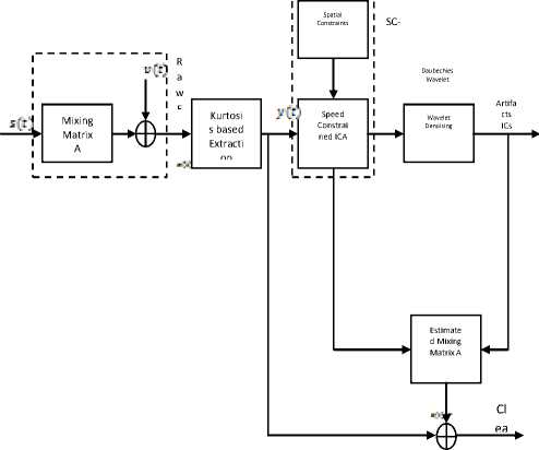
Fig.3.Overall process of artifact removal

The FastICA technique aims to maximize the statistical independence of the unconstrained sources and at the same time reducing the divergence among the spatially constrained source sensor projections and their corresponding reference topographies. A deflationary method is implemented to take out only desired components, and therefore the output of the Fast ICA technique is SC-ICs (which are artifact signals in our case), and an estimate of matching mixing matrix. This results in fast computational time, as compared with the condition that all ICs are extracted.

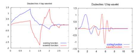
The Daubechies wavelets are a family of orthogonal wavelets defining a discrete wavelet transform and characterized by a maximal number of vanishing moments for some given support. With every single wavelet type of this class, there is a scaling function (called the father wavelet) which generates an orthogonal Multi resolution analysis.

In general the Daubechies wavelets are chosen to have the highest number A of vanishing moments, (this do not imply the best smoothness) for given support width N=2A, and among the 2A-1possible solutions the one is chosen whose scaling filter has external phase. The wavelet transform is also easy to put into practice using the fast wavelet transform. Daubechies wavelets are generally used in solving a broad range of problems, for e.g. self-similarity properties of a signal discontinuities,

signal or fractal problems, etc.

There are many Daubechies transforms, but they are all very similar. In this section we shall concentrate on the used, the Daub4 wavelet transform. The Daub4 wavelet transform is defined in essentially the same way as the Haar wavelet transform.

Transform, D4

It is assumed that S, a column vector with even number of elements, has been pre-defined as the signal to be analyzed.

N = length (S);

si = S(1:2:N-1) + sqrt(3)*S(2:2:N);

di = S(2:2:N) - sqrt(3)/4*s1 - (sqrt(3)-2)/4*[s1(N/2);

s1(1:N/2-1)];

s2 = s1 - [d1(2:N/2); d1(1)];

s = (sqrt(3)-1)/sqrt(2) * s2;

d = (sqrt(3)+1)/sqrt(2) * d1;

Inverse transform, D4

dl = d * ((sqrt(3)-1)/sqrt(2));

s2 = s * ((sqrt(3)+1)/sqrt(2));

sl = s2 + circshift(d1,-1);

S(2:2:N) = d1 + sqrt(3)/4*s1 + (sqrt(3)-2)/4*circshift(s1,1);

S(1:2:N-1) = s1 - sqrt(3)*S(2:2:N); Artifacts ICS

If a signal f has an even number N _oI values, then the 1-level Daub4 transform is the mapping f = Di ^ ( a i / d i ) from the signal f to its first trend sub-signal a 1 and first fluctuation sub-signal d1.

Each value am of ai =  (a,, . . . ,aN/2) is equal to the scalar product:

having f with a 1-level scaling signal V 1 m . Likewise, each value d m of d 1 =( d 1 , . . . , d N/ 2 ) is equal to a scalar product:

having f with a 1-level wavelet W 1 m . We shall define these Daub4 scaling signals and wavelets after briefly describing the higher levelDaub4 transforms.

The Daub4 wavelet transform, like the Haar transform, can be extended to multiple levels as many times as the signal length can be divided by 2.The extension is similar to the way the Haar transform is extended, i.e., by applying the 1-level Daub4 transform D 1 to the first trend a 1 .

This produces the mapping a 1/ D 1 → ( a 2 | d 2 ) from the first trend sub-signal a 1 to a second trend sub-signal a 2 and second fluctuation sub-signal d 2 . As with the Haar transform, the values of the second trend a 2 and second fluctuation d 2 can be obtained via scalar products with second-level scaling signals and wavelets. Likewise, the definition of a k -level Daub4 transform is obtained by applying the 1-level transform to the preceding level trend sub-signal, just like in the Haar case. And, asin the Haar case, the values of the k -level trend sub-signal a k and fluctuation sub-signal d k are obtained as scalar products of the signal with k -level scaling signals and wavelets. The difference between the Haar transform and the Daub4 transform liesin the way that the scaling signals and wavelets are defined. We shall first discuss the scaling signals. Let scaling numbers α 1 , α 2 , α 3 , α 4 be defined by

• 14-    Vs з 4- Vs s — Vs i — Vs 4V2        4V2        4-V2        4-V2

Using this natural basis, the first level Daub4 scaling signals satisfy

Цп1 = a1^2m-l+ “z^m + “a^m+l + a4^m+2

After performing above operations, the noise coefficients have minimum values, inversely to the informative signal (normal or pathologic neural activity and artifacts). Subsequently, denoising can be attained by thresholding the wavelet coefficients using Otsu’s thresholding method. The Implementation is pointed as follows:

• •    Choosing the value of the threshold using Otsu’s Thresholding Method

• •    Then daubechies wavelet transform is performed to the SC-IC signal to obtain details and approximations

• •    Threshold of the detailed components obtained in the previous step

0.05

In computer vision and image processing, Otsu's method is generally used to automatically perform histogram shape-based image thresholding, disintegration of a gray-level image to a binary image. This algorithm assumes that the image to be thresholded contains two classes of pixels or bi-modal histogram (e.g. foreground and background) then calculates the optimum threshold separating those two classes so that their combined spread (intra-class variance) is minimal. The extension of the original method for multi-level thresholding is referred to as the Multi Otsu method. This method is named after Nobuyuki Otsu.

By adaptively changing the threshold, based upon artifacts amplitude mean or variance, an optimum value could be used that would minimize the amount of undetected and incorrectly detected artifacts. By lowering the threshold, the amount of undetected blinks will decrease but it will simultaneously increase the amount of incorrect detection.

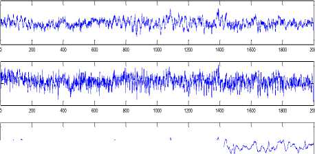
Fig.5 Control Data Amplitude (mV) vs. Sample Time (500 Hz sample

-0.05

M/h^^^^^f^

0.05

0            200            400            600            800           1000           1200           1400           1600           1800           2000

-0.05

0.05

-0.05

0.1

200            400            600            800           1000           1200           1400           1600           1800           2000

rate) after Removal; scurries indicate artifact locations.

-0.1 0

Conversely, a higher threshold will decrease false positive, but increase the chances for not detecting blinks when they occur.

• IV.    Experimental Results

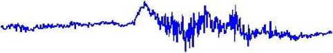
This section presents the evaluation of the proposed artifact removal technique. Initially, EEG signals are traced with occurrence of artifacts. The captured EEG signal is shown in figure2. The results obtained are depicted in figure 3 and figure 4.

Table 2. Shows the Efficiency of proposed system in case of parameters namely as peak signal-to-noise ratio and mean squared error in case different feature control data.

MSE

EEG feature PSNR

FP1	18.124567	1.0245475
FP2	17.456244	0.9646441
FZ	17.785424	0.9945875
F8	17.945465	1.1254247

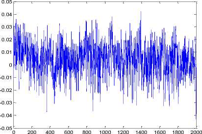
Fig 6. Original Noised Electroencephalogram Signals

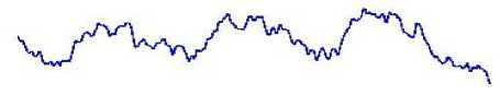
The signal resulted after the usage of wavelet Kurtosis Based Blind Source Extraction and Spatially-Constrained ICA. Final signal obtained by using the otsu’s thresholding technique is shown in figure 7 and 9. From the figures, it can be observed that the proposed artifact removal technique results in better removal of artifacts when compared to the existing technique.

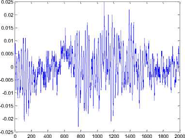
Fig 7. Final results with Conventionally Filtered transformation matrix

This would help in improving the performance of the further processing with this obtained EEG signal.

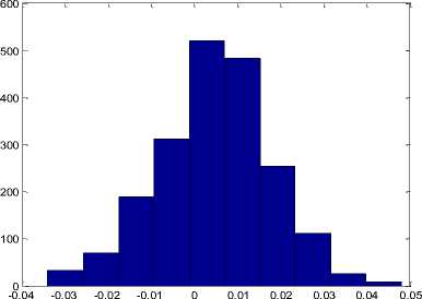
Fig.8 Shows the Histogram for the output EEG signal extracted, the results shows the values are equalized in histogram for amplitude of pure EEG signals.

Without affecting any of the data outside the location of the identified artifacts. Successful removal of this type involving accurate source separation, were found to require minimal patient movement. The third row in Figure 5 shows the independent components that were determined for this data set. The component apparently contains all of the artifacts activity with minimal activity outside of the time interval identified with the artifact occurrence.

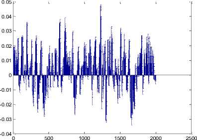
Fig 9. Shows the bar or shadow values from the extracted output values as in system developed for noise removal in Electroencephalogram signals. This will help analysis the amplitude values from patient data which is free from artifacts.

In an ideal separation of components the artifact component would be completely separate from brain activity with a waveform that consisted of the artifacts and zero everywhere else. To achieve this level of perfection an immense number of data points and recorded channels would be necessary. Because this is not achievable, the data outside of the artifact can contain minimal yet relevant brain activity. By removing only the activity in the interval identified with the artifacts occurrence in the third independent component and not the whole component, any error that could potentially be introduced by removing non-eye activity is minimized when reconstructing the signals.

Poor removal results occurred with patients that were moving or talking while data was being acquired. The removal results suffered because the Fast ICA algorithm had difficulties separating out independent sources associated exclusively with artifact activity. When sources were not separated in a fashion that resulted in one component associated with artifact activity and the removal process was performed, artifacts were attenuated instead of being removed.

• V.    Conclusion &  Discussion

This paper focuses on eradicating the artifacts from Electroencephalogram (EEG) signals. Artifact removal is a vital process earlier analyzing the EEG signal for prediction of any Compulsive diseases. Numerous scientists have focused on this process and developed their own Technique for artifact elimination. This paper intends on developing a new technique to remove the artifact from EEG. The use of daubechies wavelets and Fast ICA was successfully used in the detection and removal of artifacts, in EEG. The promising results achieved demonstrate that techniques used here are applicable to the desired task.

The proposed approach uses Kurtosis Based Blind Component Analysis (SCICA) to separate the exact Independent Components (ICs) from the initial EEG signal. After that, Wavelet Denoising is applied to extract the brain activities from purged artifacts, and finally project back the artifacts to be subtracted from EEG signals to get clean EEG data. The thresholding technique that is used in this paper is Otsu’s thresholding. Experimental evaluation suggests that the proposed approach results in better removal of artifact when compared to the existing techniques. Also, a more powerful wavelet denoising technique can be develop in order to increase results in future.