Automatic Speech Segmentation Based On Audio and Optical Flow Visual Classification

Published Online October 2014 in MECS

Automatic speech segmentation plays a major role in continuous automatic speech recognition (ASR) systems. Automatic speech segmentation consists of segmenting speech signal to the desired phonetic level. These segmented signals, then, were used to recognize spoken words in audio signals. Two major phonetic levels are mostly used in speech segmentation systems. First stage is word level in which automatic segmentation systems have to break speech audio signal into separate word segments. In this level, recognizer must support wide range of trained data as each language contains tens of thousands of words. This method is usually used for specific systems, mostly the ones which target at the implementation of voice commands recognition. Second popular segmentation level is the segmentation of phonemes. The phoneme can be described as "the smallest contrastive linguistic unit which may bring about a change of meaning"[1]. Segmenting speech signals to its phonemes help recognizer to identify a complete set of words in any language despite the fact that each language just contains tens of phonemes. Older segmentation systems used Dynamic Time Warping (DTW) as classifier [2] [3] [14] while recent methods use Hidden

Markov Models (HMMs); consequently, they have achieved more efficiency [4] [5] [15].

Performance of speech segmentation systems which only use voice signals is too much noise dependent. Some researchers used noise reduction techniques that are based on signal processing to solve this problem but they could not reach significant improvement on efficiency [20] [21] [22] [23] [24]. Thus, some new approaches use visual features from video stream of speaker’s face to reduce the effect of noise on the system performance. Akdemir et al [6] extracted some geometric features from speaker’s face and added them to audio features. They extracted those features using some blue dots which were attached to speaker lips manually while recording database. Dongmei Jiang et al [7] used some extracted geometric features from speaker lips too. They specified many points on lip contours manually and induced their features by calculating the distance between these points.

Recent researches used optical flow to detect human emotion [8] or lip reading [9]. Optical flows are some vectors that show objects motion in series of images. In this paper, optical flow vectors are used as visual features. In order to identify the features we first determined mouth area of speaker’s face using an efficient algorithm introduced by Valstar et al [10]. Then, optical flow is calculated for mouth area [11]. Next, we used another methods explained later to make a feature vector from optical flows and add them to audio feature vector. Finally, training hidden Markov model helped us to segment spoken words into phonemes.

Followings, a complete configuration of database used in this research is described. Then a deep discussion on visual feature extraction methods is given. Next, our method to extract audio features is introduced. Different fusion methods of visual and audio features are also presented. Finally, experimental results of our methods are presented and discussed.

• II.    DatabBase

The present study used VidTIMIT dataset which includes video recordings of 43 people uttering short sentences along with the correlative audio files. The whole dataset was prepared during three sessions. There was a seven-day delay between first and second sessions and a six-day delay between second and third sessions. The test section of TIMIT corpus was used as a source from which the sentences were selected. Each person was supposed to recite 10 sentences, six sentences in the first, two sentences in the second session and the other two sentences in the third session.

The participant recited identical sentences as their first two sentences, but the rest of the sentences were different for each person. The recording process was carried out in an office using a broadcast quality digital video camera. Then the resulting videos were saved as JPEG images with a 512*384 pixels resolution in a numbered sequence. The JPEG images were created using 90% quality setting. The corresponding audio is stored as a mono, 16 bit, 32 kHz WAV file.

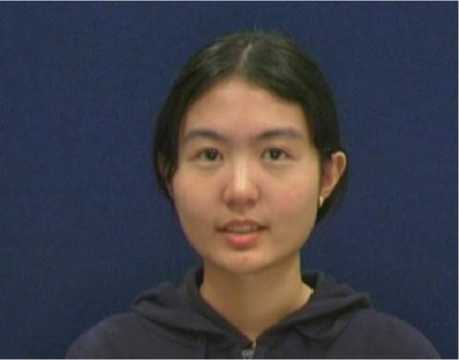
Fig 1. Example of an image in the VidTIMIT database[12]

• III.    Extracting Visual Features

• A.    Detecting mouth area

First step in extracting visual features is detecting mouth area. One possible method is detecting face of speaker and considers that his/her mouth is in the middle of bottom of his/her face. The problem is that the position and size of mouth varies for every person. So the exact position of the mouth cannot be found. Thus to find exact position of speaker mouth in image, we used an algorithm which was developed by Michel Valstar et al. Their method is more accurate in comparison with feature based [16], morphology based [17], face-texture and model based [18] and skin color based [19] techniques. Valstar used a combination of support vector regressions and markov random field to develop a method which is relatively fast and robust to moderate changes in head and face expressions. Their method first use markov random fields to find an approximate location of facial points and then support vector regressions to locate exact location of them.

• B.    Calculating optical flow

After cropping mouth area from images, optical flows are calculated for cropped area. Calculating optical flows of cropped images made our method robust to head movements across the camera surface. To calculate optical flow vectors we used Horn Schunck algorithm. [11]

The Horn Schunck algorithm assumes smoothness in the flow over the whole image. Thus, it tries to minimize distortions in flow and prefers solutions which show more smoothness. The flow is formulated as a global energy functional which is then sought to be minimized.

• IV.    Extracting Audio Features

In order to separate automatic speech segments, HMM speech recognizers were employed in forced alignment mode. In this mode, the input to the speech recognizers includes the acoustic data and the correlative transcriptions. Providing the text transcriptions helps speech recognizers by finding the phonetic boundaries; since these boundaries heighten the possibility of the input waveform occurrence. In the current study, HTK speech recognition toolkit was used to create the speech segmentation system and phonemes were chosen as the key units of segmentation system in the experiments.

The first step of using HTK should be to define the grammar that has been applied. Depending on the system, this grammar could be defined in a way that covers all the sentences of a language or a limited number of them. Since in this study, phoneme has been employed as a phonetic unit, the defined grammar must be covering all the English words and sentences. Hence, the grammar needed for the system was defined as follows:

$PHON = b | d | f | g | k | l | m | n | p | r | s | t | v | w | y | z | aa | ae | ah | ao | aw | ax | ay | ch | dh | dx | eh | er | ey | hh | ih | ix | iy | jh | ng | ow | oy | sh | th | uh | uw | zh;

([sil] < $PHON [sp] > [sil])

This means that a given list of phonemes can be put together in any possible way and there may be a pause between any of them.

Then, a list of the used words and their corresponding phonemes in the system must be defined. The application and the use of the system determine how to do this. For a simple system such as telephone dialer, the number of used words will barely outnumber the fingers. In a case that the system tries to cover all the sentences of a language, it needs to accommodate all the words of a language. Words used in this study include all the common words in the English language.

Another prerequisite for the establishment of the system is the list of uttered sentences along with the phonemes and the time of their articulation. First, the list of the sentences must be specified. The next phase would be to search the proper pronunciation in the list of words and put them and phonemes separately in different lists. HTK can also put a "sp" symbol as a sign of small pause at the end of each word, if necessary.

There are two basic approaches to consider the pause. In the first one, the pause between phonemes is not taken into account in the beginning, and it is just considered for the start and end of the sentences and then it is put between the phonemes. In the second one, the pause is considered between the phonemes and words right from the beginning. The first method is simpler and has been used. Hence, a "sil" symbol is put at the start and the end of each sentence.

The next step is to appoint the parameters of Hidden Markov Model with initial values which can also be called flat starts due to the fact that all the states have identical mean and variance. In this study, three left to right states with static 13-bit vectors along with Delta coefficients have been used. In the first stage, this model has a mean of zero and a variance equal to the initial value of one. All these definitions must be established in a file in which the initial configuration of Markov Model exists and is used as input. A corresponding model should be created for each phonetic unit.

When the overall structure of the Hidden Markov Model has been established, the parameters of the model should be given values that are closest to reality. In order to do this, training data can be used to reset the parameters. These parameters include the setting file, the file containing phonemes that have been already produced, values for threshold, the list of training file, Hidden Markov Model definitions, and the file containing phonetic files without small pauses.

Mel-frequency cepstral coefficients (MFCCs) are extracted from audio signals to train HMMs. MFCCs are coefficients that collectively make up a mel-frequency cepstrum (MFC). MFCCs result from a kind of cepstral embodiment of the audio clip and taken together, they form a Mel-Frequency cepstrum (MFC) which delineates the short-term power spectrum of a sound which is based on linear cosine transformation of a log power spectrum on a nonlinear Mel scale of frequency. In the MFCs, an equal space can be found among the frequency bands on the Mel scale. This distinguishes the regular cepstrum and the Mel-Frequency cepstrum, forasmuch as the latter is roughly closer to the human auditory system's response than the former's frequency bands' linear spaces. In audio compression, for instance, the frequency twists and turns help embody the sound better. MFCCs are commonly derived as follows:

• a)    t ake the f ourier transform of (a windowed excerpt of) a signal.

• b)    m ap the powers of the spectrum obtained above onto the mel scale, using triangular overlapping windows.

• c)    t ake the logs of the powers at each of the mel frequencies.

• d)    t ake the discrete cosine transform of the list of mel log powers, as if it were a signal.

• e)    t he mfcc s are the amplitudes of the resulting spectrum

MFCC vector of audio signal is used as audio features. What we have in the end is a proper model to get the timing and labels of the words.

• V. Integration of Audio and Vusial Information

In this section we briefly discussed about the integration of audio and visual information. In the first step, some methods which combine the average of optical flow vectors and audio information are presented. In addition, a method combining every optical flow to audio information is introduced as second step.

• A.    Average of optical flow vectors fusion with audio information

According to what was said earlier, the optical flow vectors for the rectangle surrounding the speaker's mouth are calculated. The average of these vectors is calculated in various ways and every single of them is used plus the audio data as the input for Hidden Markov Model. In the first method, the main ten spots around the mouth are taken into account including:

• 1)  Right nose hole

• 2)  Left nose hole

• 3)  Right corner of lip

• 4)  Left corner of lip

• 5)  Midpoint of upper lip

• 6)  Midpoint lower lip

• 7)  Midpoint of mouth

• 8)  Right side of chin

• 9)  Left side of chin

• 10)    Midpoint of chin

Average optical flows of six regions located among these ten points are calculated. These six regions are bounded among the following points:

• a)     1,3,5,7

• b)    2,4,5,7

c)     3,6,7

d)     4,6,7

e)     3,6,8,10

f)     4,6,910

These areas which can be seen in Figure 2 part (a) are chosen due to the fact that each of them has a different movement compared to the other parts while speaking. And it was expected that the optical flow vector illustrates the correct direction in each of them.

In the second method, twelve areas are formed by dividing each of the six areas used in the first method into two separate parts as is shown in figure 2 part (b). This is done assuming that the smaller the areas are, the less the potential errors in the calculation of the face spots would be.

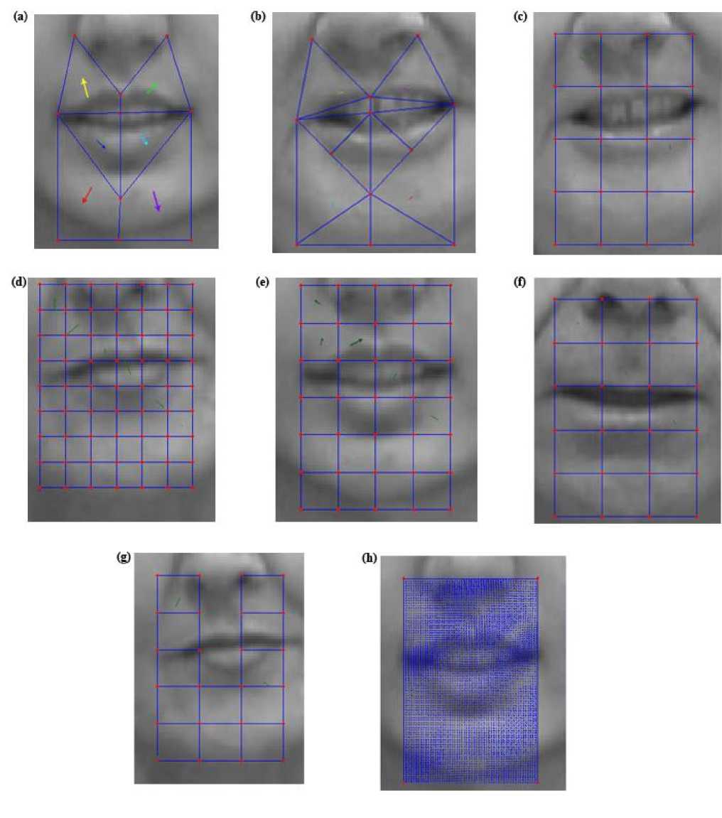
Fig 2. Deferent methods of calculating average of optical flows, (a) 6 Region; (b)6 * 2 Region; (c) 12 Region; (d) 48 Region; (e) 24 Region; (f) 15

Region; (g) 15-3 Region and (h) All vectors

• B.    Fusion of optical flow vectors average from regions with equal size with audio information

Another method used is to divide the area of the mouth into particular number of areas with the same size. In this method, the areas surrounding the mouth are specified as a rectangle which has the right corner of the lip, the left corner of the lip, the end of the nose and the end of the chin as its four edges. Then the rectangle is divided into areas with the same size. These equal-sized areas are obtained by checkering the rectangle surrounding the mouth. Several different forms are considered for the number of the areas; with 12 the least and 48 the most. Methods are also employed using 15 and 24 areas. These areas can be seen in figure 2 part (c), (d), (e) and (f).

A particular method is also used. It is like the one in which the rectangle surrounding the mouth is divided into 15 equal parts, with the difference that the three areas under the nose are omitted as it is shown in figure 2 part (g), supposing that this doesn't have much effect on the calculation, because these areas are almost motionless.

• C.    Fusion of all optical flow vectors average with audio information

  The last method employed is to use all the optical flow vectors. In this method, the rectangle surrounding the mouth which was mentioned earlier is separated and then its size is changed as it can be seen in figure 2 part (h). The standard size defined is 80 pixels high and 50 pixels wide. 4000 optical flow vectors are obtained in this process. The numbers obtained in each model are normalized and added to the vector resulting from the speaker's voice and sent as an input to Markov network.

Using audio MFCC vectors and visual features, hidden markov models are trained based on Baum Welch algorithm for every presented methods of calculating average of optical flows.

• VI.    The Exprimental Result

• A.    Method

In order to have a credible assessment of the results of the study, a consistent and specified measure must be used in assessment. One of the measures that can be used in the concept of scanning is time. If the right time of the articulation of phonemes by the speaker is available, the amounts of time obtained in the process of automatic scanning can be compared with them. The problem with this method is the need to have the exact time of the phonemes articulation. Due to the fact that this information didn't exist in the used database and the calculation wasn't possible either, regarding the potentiality of human error and being time-consuming, this measure couldn't be used for assessment. Another measure widely used in similar studies is WACC or accuracy in word recognition. In this study, phonemes were divided into groups, each of which includes phonemes that are articulated in a similar way. For instance, the form of lips and mouth while articulating the phonemes "m" and "b" is the same. Therefore, these two phonemes are categorized in one group. The classification used, consists of five major categories which in turn include all the articulable phonemes by the human being. The vowel phonemes are divided in two groups. In the articulation of the first group of vowels, lips get round and the rest of the vowels go to the second group. The consonant phonemes are divided in three groups. The first group is composed of those consonants which are articulated by sticking the lips or teeth together. The second group consists of those consonants that are articulated inside the mouth and the third group contains phonemes articulated inside the pharynx.

• B.    Experimental Results

The presented method is tested for sounds with different noises. First, noiseless sounds are tested whose result of use in different methods can be seen in table I. As the table illustrates, the noiseless sounds without an image have been recognized reasonably. Although, the use of some image-included techniques is helpful in the improvement of the recognition, even slightly, some of them are weakened the recognition, in comparison with the cases in which no image is used. This probably happens because the amount of visual data exceeds the audio data and this leads to the dominance of visual input to audio input and hence the recognition process undergoes a disorder. Best results are obtained when 15 visual vectors are used. Subtracting three vectors out of fifteen vectors didn't have a positive effect on the recognition and cut it a bit. The use of 24 vectors instead of 15 vectors is of no use, either. The use of visual vectors, when there is little noise, hasn't had such a conspicuous improvement and all in all, it doesn't seem to be effective, regarding its overall calculation.

Table 1. Wacc for different methods And SNRs

Method	WAcc
	No Noise	SNR 15	SNR 5
Audio Features Only (AF)	93%	68%	54%
AF + 6 Visual feature	94%	69%	61%
AF + 6 * 2 Visual feature	94%	87%	80%
AF + 12 Visual feature	94%	69%	66%
AF + 15 - 2 Visual feature	95%	91%	85%
AF + 15 Visual feature	96%	92%	86%
AF + 24 Visual feature	95%	91%	83%
AF + 48 Visual feature	91%	78%	59%
AF + all optical flows	89%	75%	58%

Just like noise-free signals, use of a large number of visual data has a slight improvement. The noticeable point about recognition with this amount of noise is the insignificant effect of the use of average of vectors surrounding the mouth with 6 part divisions set to the face spots in comparison with methods with fixed division. The reason for this shortcoming probably is that this method is strongly dependent on the spots of the face and the slightest error in the recognition of face spots leads to error in the resultant optical flow vectors calculation and decreases the efficiency. Doubling the appointed areas of the face hasn't brought up much difference with the original form of this method. Comparison of this method with the method which employs 12 fixed parts reveals that although the number of the areas is the same, the method with fixed classification is more efficient which is probably due to the errors in the calculation of face spots.

When the sound signal has a ratio of signal to noise equal to 5, with the use of audio data without visual data, the recognition has been low. A point worthy of notice in this table is that the use of all visual vectors which lowered the recognition in noise-free cases compared to the techniques without the image, has been more efficient rather than method with mere use of audio data. This may have happened because of too much noise in the audio data, in a way that they had been less efficient compared to mere visual data.

• VII.    Conclusion

In this paper we presented a novel method for bimodal speech segmentation which made speech segmentation more robust due to the noise in comparison with other existing methods. Different methods of extracting visual features based on optical flow calculation of mouth area were developed. Among presented segmentation systems with different methods, those which use audio and visual features increased accuracy of detection in comparison to the same system which use audio features only. We showed that using optical flow vectors from speaker’s mouth can increase noise robustness. Some methods of extracting visual features need more facial points.

Through the experimental results, we demonstrated that methods which need less facial points are more accurate. This implies that making optical flow average calculation dependent to facial points can harm accuracy. This is because facial point position calculation contains errors. Our method also needs high quality image sequence of speaker’s face during speech; which is not always available.