Automating the Process of Work-Piece Recognition and Location for a Pick-and-Place Robot in a SFMS

Vision systems find profound usage in automation of industrial processes and associated research. Some of these include burr measurement [1], inspection of surface texture [2], grading and sorting food products [3], amongst others. Recognizing and locating objects or work-pieces in a manufacturing workcell is another such application which is essential in automating pick-and-place operations.

Such automation work can also be used as an education tool to demonstrate flexible manufacturing concepts to students as seen in the works of Nagchaudhuri in [4-6]. In [5, 6], students carried out a project requiring them to use a SCARA robot, which was fitted with a two finger gripper, to manipulate the arbitrary placed letters H, E, L (two), O from the workplane of the robot to predefined locations to read HELLO. The work-plane of the robot was covered by an overhead CCD camera and the students were required to develop appropriate software programs to recognize the letters and then achieve the above task.

While there are already off-the-shelf packages available for such applications, they are normally very costly and require specialized software and hardware maintenance when task specific, low-cost, easily maintainable vision systems are often desired. This work presents development of such a vision system to automate the process of work-piece recognition and location for an in-house developed pick-and-place robot.

The developed system is part of a smart flexible manufacturing system (SFMS), the framework for which is shown in Figure.1. The system is termed smart because it can be accessed and controlled globally from remote locations by authorized users. The machining center consists of a CNC drilling machine [7]; the transportation system is an automatic guided vehicle (AGV) which uses infra-red (IR) sensors to follow the guide path on a manufacturing shop floor while using an obstacle avoidance algorithm to avoid obstacles [8]; the remote machining system is based on Internet technology such that the CNC drilling machine could be controlled by registered and authenticated users from any part of the globe [9]; and the vision-based pick-and-place system is reported in [10-12].

The vision system is integrated into the workspace of the pick-and-place robot to recognize the shape and color of work-pieces on the work-plane of the robot along with their location. Work-pieces with user specified shape and color will then be unloaded to the workstation from the AGV for drilling operations. The system overview and the development of the vision system are explained in section II and section III respectively followed by discussion in section IV and the conclusion in the last section.

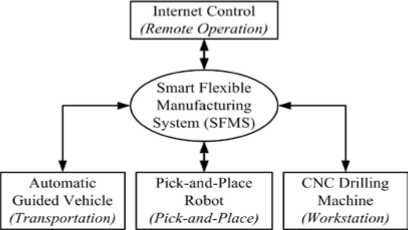
Figure 1. Framework of the SFMS

• II.    SYSTEM OVERVIEW

The framework for the developed system is shown in Figure.2. The five degree-of-freedom (DOF) pick-and-place robot for this work is designed for handling light weight and small size material such as wood and aluminum and therefore has a limited payload of 500 g. The vision system includes an overhead mounted camera that covers the work-area of the robot. System operation is through a graphical user interface (GUI) which allows the user to input the shape and color of the work-piece(s) to be manipulated by the robot. On user input, a snapshot of the work-plane is taken and image processing is performed to determine the shape and color of the workpieces. Work-pieces with three possible shapes: rectangle , circle , and triangle ; and five possible colors: red , green , blue , yellow , and black are scattered on the rectangular work-plane of the robot. Along with their shape and color, the location of the work-pieces on the work-plane is also determined to perform the pick and place operations.

The robot is controlled by a peripheral interface controller (PIC) which allows easy interface to the control electronics. However, for motion planning and since the overall project also involves vision processing, sufficient additional processing power is provided in the form of a personal computer (PC), designated as a server. Output data from motion planning is communicated on request through the enhanced parallel port (EPP) of the PC to PIC microcontroller, acting as the client, which actuates the robot and interfaces with the sensing devices. The client-server control architecture is explained in [12].

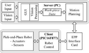
Figure 2. Framework for the vision-based pick-and-place robot

• III.    VISION SYSTEM

An overview of the vision system adapted for this work is given in Figure.3. Since the setup is located in an indoor environment, the scene constraints in this context mainly refers to uneven lighting that surrounds the vision system hardware. Removal of this noise makes image pre-processing simpler and, therefore, a lighting system is designed.

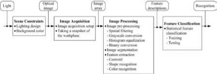
Figure 3. Overview of the vision system

Image acquisition refers to the retrieval of image from the image acquisition hardware while image preprocessing is performed to remove unwanted data or noise from the image. Image segmentation separates the objects in the image from the background which facilitates the process of feature extraction. Since image pre-processing, image segmentation, and feature extraction require processing of the captured image, these subsystems are referred as the steps involved in image processing. After the extraction of features, a feature classification subsystem classifies them for shape and color recognition.

A.    Scene Constraints

Scene constraints are the first and probably the most important element in any vision system. It refers to the environment that the vision system will be subjected to which in turn depends on the application. The aim is to reduce the complexity of the captured image so that fewer processing is required at subsequent sub-systems in Figure.3.

Two most critical factors that influence a captured image are the lighting system and the color of the workplane, the background on which the work-pieces are scattered. The ideal choice for the color of the work plane is either black or white. This is because the work-pieces are easily separable from black and white colored background during image segmentation. Since the workpieces also have a possible black color, the color of the work plane is limited to white. The vision unit also includes a structured lighting system with one 11 Watt compact fluorescent lamp placed on each side of the camera to minimize specular reflections and shadows around the work-pieces.

B.    Image Acquisition

The vision unit consists of an overhead mounted CCD camera (Sony digital video camera (model DCR HC42E)) which is connected via the universal serial bus (USB) port to a PC which has a 2.4 GHz processor and 512 Mbytes of random access memory (RAM) running under the Windows XP operating system. The camera has a

CCD size ¹₅" and an image size of 320×240 pixels covering a rectangular work-plane with dimensions 348.14×261.11 mm, determined using the maximum and minimum reach of the robot. The rectangular view of the work-plane as seen by the camera is streamed into the PC and a single snapshot image, which is in the RGB color model with 8-bit of data, is taken for processing on user input through the GUI.

C. Image Processing

Image Pre-processing

Image acquisition is followed by image pre-processing. The steps in image pre-processing that were utilized for this work are spatial filtering, grayscale conversion, histogram equalization, and binary conversion. Feature extraction for shape recognition is performed using the binary image while the spatial filtered image is used for color recognition.

Spatial filtering is the direct manipulation of the pixels in the image on the image plane itself and is denoted by the expression

condition that T g must be monotonic and c 1 ( T g ( a )) should not overshoot c 0 ( a ) by more than half the distance between the histogram at counts a .

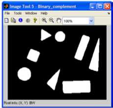
The histogram equalized grayscale image, g e , is then converted to binary format. The binary image has pixel values as either 0 (black) or 1 (white). A threshold, T b , is determined such that a normalized pixel value below it is converted to 0 and above it is converted to 1. That is, the binary image, b , is defined as

b ( ^x , y ) =

if g e ( ^x , У ) > T b if g e ( ^x , У ) < T b ^.

The threshold is determined using Otsu’s method [15].

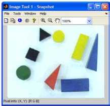
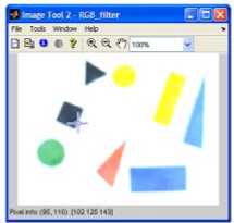
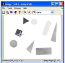
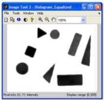
A sample captured image in the RGB color model, the spatial filtered RGB image, the grayscale image, histogram equalized grayscale image and its binary image (the complement of the binary image taken in this case) are shown in Figure.4.

f o ( X , У ) = T n [ fl ( X , y )]

Where f i ( x , y ) and f o ( x , y ) are the input and output images respectively [13]. In addition, T n , an operator on f i , is outlined about the point ( x , y ) over a specified neighborhood. The best results for the output image was obtained using a 7×7 correlation kernel with coefficients of 0.04.

The image is then converted to grayscale format, also known as an intensity image, which in this case is represented using 8-bit data and has pixel values ranging from 0 to 255, where 0 represents black and 255 represents white. Grayscale values are same as the luminance (Y) of the YIQ color space [13] and are obtained from the RGB components of the filtered image through the transformation

Y

I

Q

0.299

0.596

0.211

0.587

- 0.274

- 0.523

0.114

- 0.322

0.312

R

G

B

The grayscale image often has most of its intensity values concentrated within a particular range which requires histogram equalization. This enhances the contrast of the image by transforming the intensity values of the grayscale image so that the histogram of the output image has the intensity values evenly distributed. Therefore, a grayscale transformation T g is found such that to minimize

I c i ( T g ( k )) - c o ( k )|

Where c 0 is the cumulative histogram of the grayscale image and c 1 is the cumulative sum of the desired histogram for all intensities k [14]. This is subject to the

(a)

(b)

(c)                                (d)

(e)

Figure 4. (a) Captured RGB image, (b) RGB image after spatial filtering, (c) grayscale image, (d) histogram equalized grayscale image, and (e) binary image

Image Segmentation

Image segmentation partitions an image into meaningful regions which correspond to objects of interest in the image. From the binary image, the workpiece pixels are represented as white and the background

pixels as black and, therefore, white pixels which are connected to each other denote a single work-piece.

Feature Extraction

This work involves recognition of shape and color of work-pieces and, therefore, features that differentiate both shape and color are discussed. Shape recognition is based on the 2D image of the work-pieces, that is, 2D shape recognition. Features such as roundness, radius ratio, and the number of corners were explored for shape recognition while the hue, saturation, and value of the HSV color model are used for color recognition. The computation of the centroid of the work-piece is also presented which is used to determine the location of the work-piece on the work-plane.

Feature Extraction: Centroid

The moment of the work-piece is used to determine its centroid. The basic equation that defines the moment of order (i+j) for a two-dimensionsal continuous function f(x,y) is given in [16, 17] as mij = J -oof —0 ^У1 f (X, У ) dX dy .                   (5)

For a digital binary image, this can be rewritten as mil = ZZ x^f (x, у)                          (6)

xy

Where x and y represent the pixel coordinates of the binary image and f ( x , y ) denotes the corresponding pixel value.

Using moments, the x and y coordinates of the centroid are expressed as x = m10   and y = m01                    (7)

m ₀₀               m ₀₀

Where m 00 denotes a zero-order moment, and m 01 and m 10 denote first-order moments.

This coordinate is then transformed to the robot coordinate system through camera calibration before applying inverse kinematics to determine the robot arm positions for picking the work-piece as given in [10, 11].

Feature Extraction: Shape Recognition

Two different methods, a combination of roundness and radius ratio, and the number of corners were considered for shape recognition with the latter found to be more efficient.

Roundness, sometimes also referred to as compactness, is defined as

outline of an object, with continuous boundary is defined as

P = J V x ²( t ) + y ²( t ) dt

Where t is the boundary parameter. However, for a digital binary image, this can be modified to

Z

^P = Z V( x z + 1 ^- x z ) ⁺( У г + 1 ^- У г ) z = 1

Where z = 1, 2, 3, … , Z denotes the coordinate set of the boundary pixels of a single work-piece in the binary image.

In a binary image, the area of a single work-piece can be defined as number of pixels that represent that workpiece.

Similarly, radius ratio, also referred to as a measure of eccentricity or elongation, is defined as

d min

^Rr = m--- d max

Where d min and d max denote the minimum and maximum distances to the boundary from the centre of the work-piece respectively. Thus, for all the boundary pixels, the distance from the centre of a work-piece is given as

^dz =^ ( У z ^- У ) ^{2 +} ( x z ^- x ) ² .                        ⁽¹²⁾

The pixel with coordinates ( x min , y min ) has minimum

distance to the centroid if

d min <  d_z     ^ z, z ^ min .

Similarly, a pixel with coordinates ( x max , y max ) has

maximum distance to the centroid if

d™ x >  d₇    V z , z ^ max.

max z         ,

The number of corners is another feature for shape recognition and it is a very realistic approach to the problem of shape recognition as it is usually the number of sides or corners that humans use for differentiating shapes. A corner, as defined in [18], is a location on the boundary of an object where the curvature becomes unbounded and is given as

R = pL

4 n A

k ( t ) ²

2² d_X [ dt ² J

2² dx

,

Where P and A refer to the perimeter and area of the work-piece respectively [18]. Perimeter, the length of the

Where t represents the distance along the boundary of the segmented regions and a corner is declared whenever | k ( t )| assumes a large value.

Eq. 15 can be modified for a digital binary image. If

A x_z

= ^xz + 5 - ^xz

And

^A y z = y z + 5 - y z

Where x z and y z are the x and y coordinates of the boundary pixels, s is the sample length of the curvature and with the approximation that the length of the curvature is given by

A t z = ^Ax z ² +A y z ² ,                             (18)

the curvature of a digital binary image is given as

^A y z + 1

^A t z + 1

^A y z I _J_|^{A x}z + 1    ^{A x}z

I + I

^A t z )   U t z + 1    ^A t z

Feature Extraction: Color Recognition

Color, as defined by [19] is how one interprets light and is something which is invariant with respect to light intensity. Colors are interpreted as the varying components of the primary red ( R ), green ( G ), and blue ( B ) components of the color space, as shown in Figure.5, which can be easily transformed into other color spaces.

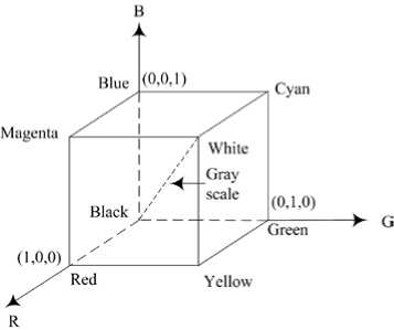
Figure 5. The RGB color cube

Some commonly used color spaces for digital image processing are the basic RGB color space, the CMY and CMYK color spaces, the XYZ color space, and the HSV and HSI color spaces. The RGB color space is not preferred in inconsistent environments due to the varying R , G , and B components of the capturing device [17, 19]. Cyan ( C ), magenta ( M ), and yellow ( Y ), also known as the secondary colors of light, are additions of the primary colors. A further addition of the black color to the CMY color space produces the true black color referred to as the CMYK color space. The amount of red, green, and blue required in the formation of a color, known as the tristimulus values, are denoted as X , Y , and Z respectively.

A color is then represented by its trichromatic coefficients , x , y , and z , which are defined from the tristimulus values. In image processing, the XYZ color space is taken as rather supplementary.

The HSV (hue, saturation, and value) and HSI (hue, saturation, and intensity) color spaces are a more natural way to how humans perceive color and is more often used for color image processing. As such, the HSV color space was used for representing the features for color recognition in this work. The HSV model is also sometimes referred to as tint, shade, and tone and has colors defined inside a hexcone as shown in Figure.6(a) with the positioning of the hue and saturation in the model, for an arbitrary point, shown in Figure.6(b). Hue describes the color type given as an angle from 0° to 360°. Typically 0° is red, 60° is yellow, 120° is green, 180° is cyan, 240° is blue, and 300° is magenta. Saturation is the purity of a color or the amount of white added to the color and has values from 0 to 1 where S = 1 specifies a pure color, that is, no white. Value is referred to as the brightness of a color and ranges from 0 to 1, where 0 is black.

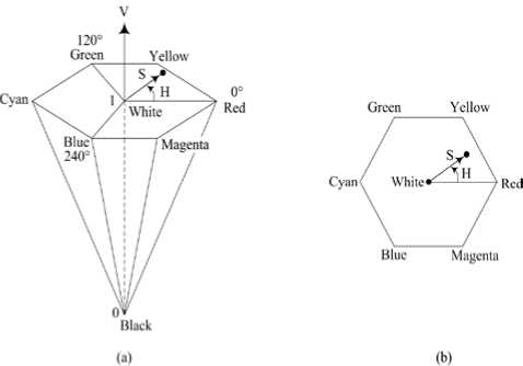
Figure 6. (a) The HSV color model, and (b) hue and saturation in the HSV color model. The dot is an arbitrary color point

The transformation from the RGB color space to the HSV color space is given in [20] as

G - B

60 x          + 0 , if Max = R and G >  B

Max - Min

G - B 60 X----------

Max - Min

B - R 60 X----------

+ 360 , if Max = R and G <  B

H = i

S =

Max - Min

R - G

60 X----------

Max - Min

Max - Min

+ 120 , if Max = G

+ 240 , if Max = B

Max

V = Max

Where Min = min(R,G,B) and Max = max(R,G,B) with normalized values of R, G, and B used.

C.    Feature Classification

The statistical feature classifier [21], as shown in Figure.7, is operated in two modes: training (learning) and testing (classification). In the training mode, a database of images is built that contains known shape and color of work-pieces. The knowledge gained from the extracted features forms the database with which the classifier is trained to distinguish the different feature classes in the feature space. An input feature vector is then classified into one of the feature classes depending on its measured features.

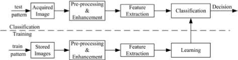
Figure 7. Model of a statistical feature classifier

Since the number of shapes and colors to be differentiated is three and five respectively, there are fifteen possible feature classes. The four-dimensional mean feature vector, m j , is represented as

C

H

S

V

Where C denotes the number of corners and H , S , and V the hue, saturation, and value for the j ^th class respectively.

In the testing phase, an input feature vector, obtained from a test image, is to be assigned to one of the fifteen feature classes. The classification technique is based on decision-theoretic approach. In decision-theoretic approach, also known as decision or discriminant function approach, an input feature vector gives different responses when operated on separate feature classes. From [13, 17], if x = (x1, x2, …, xn)T represents an n-dimensional feature vector, then for J feature classes j1, j2, …, jJ, this approach finds J decision functions d1(x), d2(x), …, dJ(x) such that if x belongs to class ji, then di (x)> d j (x) , V J j * i. (22)

That is, an unknown feature x is assigned to the i th feature class if d i ( x ) returns the largest numerical value after substitution in all decision functions.

Various recognition techniques, such as minimum distance classification, probabilistic approaches, and neural network are used as decision functions. However, due to the distinct nature of the feature classes, the simplest approach of minimum distance classification is utilized. The distance here refers to the Euclidean distance which is determined as dj (x) = ||x - m j||

Where || a ^ = ( a T a )¹ / ² is the Euclidean norm [13, 17].

• VI. DISCUSSION

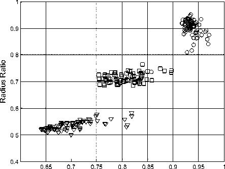
For shape recognition, initially roundness and radius ratio features were experimented with. Figure.8 shows the clustering of the two features using training data. In Figure.8(a), the rectangle and triangle had approximately equal length for all the sides, that is, square and equilateral triangle, which resulted in easily separable clusters. However, with the ratio of the length of the sides varying for the rectangle and triangle, the clusters were overlapping for these two shapes, as shown in Figure.8(b). This resulted in incorrect classifications during testing for these two shapes especially with increasing ratios between the dimensions for each side.

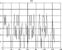
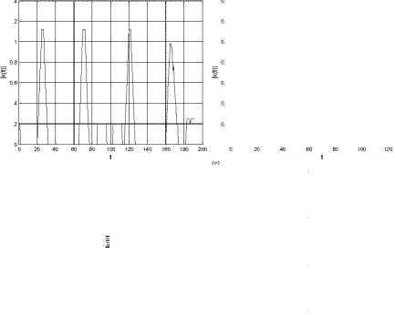
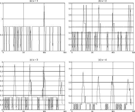
This prompted the use of the number of corners as the feature for shape recognition. In implementing the corner detection algorithm, sample length, s , from 1 to 5 pixels was experimented with. The curvature of a rectangle sampled at varying sample lengths is shown in Figure.9.

Generally, it was difficult to determine the correct number of corners at lower values of s . After performing similar analysis for different shapes with different length of the sides of the shapes, a sample length of five pixels was determined as the optimum one. The curvature for a sample rectangle, circle, and triangle sampled at five pixels is shown in Figure.10. The four and three outstanding peaks in Figure.10(a) and Figure.10(c) correspond to the corners of a rectangle and a triangle respectively. For a circle, Figure.10(b), the non-presence of any outstanding peak implies the non-presence of corners.

(a)

Roundness

(b)

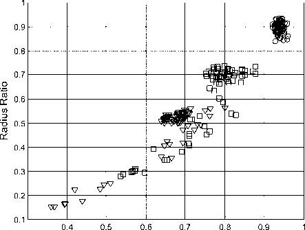
Roundness

Figure 8. (a) Clustered features for rectangle and triangle for sides with approximately equal length, and (b) clustered features for rectangle and triangle with sides of different length (Note: The plot shapes correspond to the shape of the workpiece)

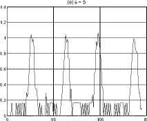
Figure 9. Curvature of a rectangle at different sampling lengths

For color recognition, the HSV values for a single work-piece are averaged from 16 random pixels between the x and y limits of an inscribed square in an inscribed circle as illustrated for a rectangle, triangle, and circle in Figure.11 (a), (b), and (c) respectively. The inscribed circle has a radius equal to the minimum distance from the center of the work-piece to its boundary as determined when calculating the radius ratio.

With reference to the dashed line that represents a circumscribed square, the random points selected within the x and y limits may assume values outside the boundary of the work-piece, resulting in inaccurate values for color description. Thus, an inscribed square is preferred with the resulting vector diagram as shown in Figure.12 where x l , min and x l , max , and y l , min and y l , max denote the minimum and maximum limits in the x and y directions respectively.

(a)

1.4

1.2

0.6

0.4

0.2

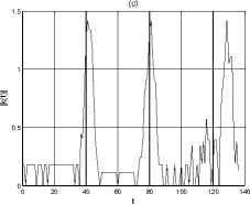
Figure 10. Curvature for a sample (a) rectangle, (b) circle, and (c) triangle

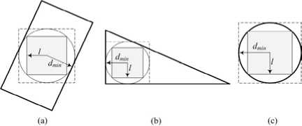
Figure 11. Inscribed square for (a) rectangle, (b) triangle, and (c) circle

The value of l can then be determined as

l = d min 2

.

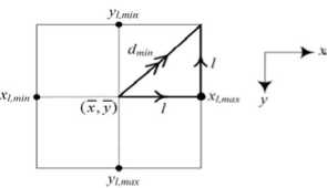
Figure 12. Inscribed square with vector components

The minimum and maximum limits in the x and y directions for calculating the random points are then given as

( x - 1 ) < x < ( x + 1 ) (25)

And

( У ^{- 1} ) < У < ( У ^{+ 1} )

respectively.

The 16 random points for each work-piece that were used to approximate its color for the captured color image in Figure.4 are shown in Figure.13.

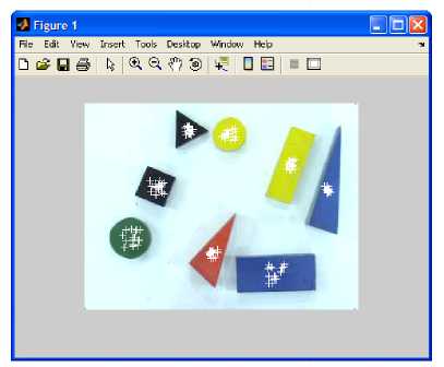
Figure 13. Scatter of the 16 random points for each work-piece for color recognition

The mean HSV color values of a particular work-piece is then determined as

HSV =

K

^X H ( x k ^, У к ) к = 1

K

K

^X S ( x k ^, У к ) к = 1

K

K

^X V ( x k , У к ) к = 1

K

where K is the number of random points, 16 in this case.

For shape recognition, the a priori knowledge on the number of corners is utilized. However, for color recognition, the mean H , S , and V color values are obtained to represent the feature vector for a class. The training phase is composed of five images of each class resulting in a total of seventy five images, with each image containing three work-pieces of the same class.

A scatter of the RGB values of each colored workpiece in the RGB color space from the training phase is shown in Figure.14. However, the RGB color space produced inconsistent results with slight changes in surrounding such as number of work-pieces on the workplane and the light intensity or ambient light. The HSV color space was found to give better results and was utilized as a result. The mean feature vector for the fifteen classes is given in Table I with the H , S , and V values normalized.

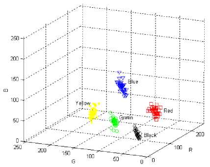
Figure 14. Scatter of the RGB color values for each color (the plot color corresponds to the respective color)

TABLE I. MEAN FEATURE VECTOR FOR THE FIFTEEN FEATURE CLASSES

j	Class, j	Mean Feature Vector, m j
1	Red rectangle	[ 4 0.0271 0.7260 0.6816 ]
2	Green rectangle	[ 4 0.3850 0.4984 0.3454 ]
3	Blue rectangle	[ 4 0.6184 0.6661 0.5603 ]
4	Yellow rectangle	[ 4 0.1824 0.8967 0.7561 ]
5	Black rectangle	[ 4 0.5354 0.2304 0.2245 ]
6	Red circle	[ 0 0.0271 0.7260 0.6816 ]
7	Green circle	[ 0 0.3850 0.4984 0.3454 ]
8	Blue circle	[ 0 0.6184 0.6661 0.5603 ]
9	Yellow circle	[ 0 0.1824 0.8967 0.7561 ]
10	Black circle	[ 0 0.5354 0.2304 0.2245 ]
11	Red triangle	[ 3 0.0271 0.7260 0.6816 ]
12	Green triangle	[ 3 0.3850 0.4984 0.3454 ]
13	Blue triangle	[ 3 0.6184 0.6661 0.5603 ]
14	Yellow triangle	[ 3 0.1824 0.8967 0.7561 ]
15	Black triangle	[ 3 0.5354 0.2304 0.2245 ]

During final experimentation, work-pieces were randomly placed on the work-plane of the robot and each time their shape, color, and location was successfully determined.

• V. CONCLUSION

The development of a vision system for automating the process of work-piece recognition and location for a pick-and-place robot has been presented. It includes an overhead mounted camera and on user specification of the shape and color of work-piece to be manipulated by the robot, a single image is acquired into the PC for further processing. The number of corners are then determined through image processing to determine the shape of the work-pieces while the hue, saturation, and value of the colors are used to determine the color of the work-pieces. This work, however, does not look at the case of touching and overlapping work-pieces which is planned as future work.

ACKNOWLEDGMENT

This work was funded by the University Research Committee at the University of the South Pacific under research grant 6C066.