Basic definitions of quantum computing of IT students in intelligent cognitive control and robotics

Author: Reshetnikov Andrey, Tanaka Takayuki, Tyatyushkina Olga, Ulyanov Sergey
Journal: Сетевое научное издание «Системный анализ в науке и образовании» @journal-sanse
Article in issue: 3, 2017.
Free access
Quantum computations results from the link between quantum mechanics, computer science and classical / quantum information theory. It uses quantum mechanical effects, especially superposition, interference and entanglement, to perform new types of computation which show promise to be more efficient than classical computations. It is the essential trait of the theory of quantum mechanics to make (exclusively) probabilistic predictions, i.e. for a quantum mechanical experiment the theory predicts possible results and their probabilities to occur. This is what makes quantum computing probabilistic.
Quantum computing, quantum operators, probabilistic inference
Short address: https://sciup.org/14123272
IDR: 14123272
Основные понятия квантовых вычислений для студентов ИТ интеллектуального когнитивного управления и робототехнике
Квантовые вычисления основаны на законах квантовой механики, компьютерных технологий и теории информации. При этом применяются квантово-механические эффекты, особенно суперпозиция, интерференция и запутанные состояния, порождая новые типы вычислений, которые являются более эффективными при поиске решений, чем классические вычисления. Особенностью такого рода вычислений является вероятностная природа предсказания ожидаемого результата в силу физической природы законов квантовой механики. Это приводит к вероятностной природе квантовых вычислений и квантовых алгоритмов.
Text of the scientific article Basic definitions of quantum computing of IT students in intelligent cognitive control and robotics
ОСНОВНЫЕ ПОНЯТИЯ КВАНТОВЫХ ВЫЧИСЛЕНИЙ ДЛЯ СТУДЕНТОВ ИТ ИНТЕЛЛЕКТУАЛЬНОГО КОГНИТИВНОГО УПРАВЛЕНИЯ И РОБОТОТЕХНИКЕ
Решетников Андрей Геннадьевич1 , Танака Такаюки2 , Тятюшкина Ольга Юрьевна3 , Ульянов Сергей Викторович4
1Доктор информатики (PhD in Informatics), к.т.н., доцент;
ГБОУ ВО МО «Университет «Дубна»,
Институт системного анализа и управления;
141980, Московская обл., г. Дубна, ул. Университетская, 19;
2Доктор наук (PhD in Engineering),
Высшая школа информатики и технологии,
Университет Хоккайдо;
N14, W9, Саппоро-Ши, Хоккайдо, Япония;
Институт системного анализа и управления;
141980, Московская обл., г. Дубна, ул. Университетская, 19;
4Доктор физико-математических наук, профессор;
ГБОУ ВО МО «Университет «Дубна»,
Институт системного анализа и управления;
141980, Московская обл., г. Дубна, ул. Университетская, 19;
The interplay between mathematics and physics has always been beneficial to both fields of endeavor. The calculus was developed by Newton and Leibniz in order to understand and describe the dynamics of motion of material bodies. In general, geometry and physics have had a long and successful symbiotic relationship: classical mechanics and Newton’s gravity are based on Euclidean geometry, whereas in Einstein’s theory of general relativity the basis is provided by non-Euclidean Riemannian geometry (an important insight taken from mathematics into physics). Although this link between physics and geometry is still extremely strong, one of the most striking connections today is between information theory and quantum physics.
Long time we have not though about computation in physical terms. We considered the computation from the standpoint of mathematics and connected it with the notion of algorithm and Turing machine. But computation itself carried out by means of a physical process in a computing device. Computers today become not only faster, they become smaller too. At some stage of miniaturization it is necessary to include in the description of computers a quantum phenomena (Manin, 1980; Feynman, 1982). Deutsch (1985) considered a situation where computers like quantum objects can enter highly non-classical states. These quantum computers could, for example, exist in a superposition of states.
Computation, based on the laws of classical physics, leads to different constraints on information processing than computation based on quantum mechanics. Quantum computers hold promise for solving many intractable problems, but, unfortunately, there currently exist no algorithms for “programming” a quantum computer. The interplay between mathematics and physics has always been beneficial to both fields of endeavor. The calculus was developed by Newton and Leibniz in order to understand and describe the dynamics of motion of material bodies. In general, geometry and physics have had a long and successful symbiotic relationship: classical mechanics and Newton’s gravity are based on Euclidean geometry, whereas in Einstein’s theory of general relativity the basis is provided by non-Euclidean Riemannian geometry (an important insight taken from mathematics into physics). Although this link between physics and geometry is still extremely strong, one of the most striking connections today is between information theory and quantum physics.
Calculation in a quantum computer, like calculation in a conventional computer, can be described as a marriage of quantum hardware (the physical embodiment of the computing machine itself, such as quantum gates and the like), and quantum software (the computing algorithm implemented by the hardware to perform the calculation). To date, quantum software algorithms, such as Shor’s algorithm, used to solve problems on a quantum computer have been developed on an ad hoc basis without any real structure or programming methodology.
The lack of a quantum programming or program design methodology for quantum computers severely limits the usefulness of the quantum computer. Moreover, it limits the usefulness of the quantum principles, such as superposition, entanglement and interference, that give rise to the quantum logic used in quantum computations. These quantum principles suggest, or lend themselves, to problem-solving methods that are not typically used in conventional computers.
Quantum principles and quantum logic can be used with conventional computers if we find solutions to simulate and implement quantum algorithms in classical computers. The present paper describes solutions of these and other problems by providing method of simulation and design of quantum algorithm gates to implement quantum algorithms for quantum computing and quantum soft computing that can be classically efficiently simulated.
The interrelations between physics, mathematics and informatics from quantum paradigm point of view is shown in Fig.1. In theoretical backgrounds part we briefly introduce main concepts and ideas of topics depicted on Fig.1.
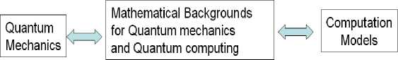

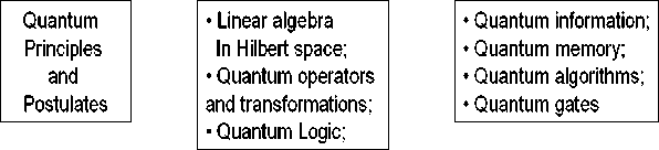
Figure 1. Background of quantum computing
Let us consider a usage of quantum computation ideas for our task formulated above.
The quantum principles (such as quantum parallelism, quantum complementary, quantum long-distance correlation, quantum bio-inspired searching, etc.) can be used for applications of quantum strategies for optimal decision making with conventional computers in much the same way that genetic principles of evolution are used in genetic optimizers. Nature also uses the principles of quantum mechanics to solve problems, including quantum-like optimization-type problems, searching-type problems, selection-type problems, etc.
The quantum operators , such as superposition, entanglement and interference , give rise to the quantum logic used in quantum computations. Moreover, the usefulness of these quantum operators gives rise to the new viewpoint on control and self-organization algorithms.
In the classical computation one bit information is coded as 0 or 1. We can say also that one bit of information can represent the state 0 or the state 1. In quantum computation quantum state information is used as a superposition of two states ( a 10) + a 11 ) and it is called as qubit (quantum bit).
With superposition operator for a given algorithm we can introduce all initial states that include the searching solutions, and accelerate computation processes by massive quantum parallelism.
The entanglement operator has no analog in classical computation. It allows physically set up statistical relations (quantum correlations) between solutions on the searching of space of the algorithm. In particular important case, it is the physical source of quantum oracle algorithms.
The interference operator performs division of solutions obtained by the quantum algorithm by finding a successful solution with maximal probability amplitude.
Quantum principles and quantum logic can be used with conventional computers if we find solutions to simulate and implement quantum algorithms on classical computers.
Remark . That does not mean that deterministic quantum computations are impossible, but that the nature of quantum computing is based on probabilities.
This article describes the fundamental principles of quantum computing from engineering point view. It introduces the quantum circuit model of computation, which provides a “language” to describe quantum algorithms and explains its basic building blocks: quantum bits, quantum operations (gates) and quantum measurements [1-18].
The mathematical framework describing the concepts and principles of quantum mechanics is of course also the theoretical basis of quantum computing. Therefore, it is necessary to deal with the basic postulates of quantum mechanics which connect the physical world with its mathematical model. These postulates directly relate to the modeling of the key elements of quantum computation:
-
• compositions of such systems,
-
• operations on quantum systems for the purpose of information processing, and
-
• the readout (measurement) of information from quantum systems.
Within this introduction the postulates of quantum mechanics are specified in the subsections dealing with the corresponding topics.
Basic knowledge of linear algebra and the tensor product is assumed, but the necessary mathematics can also be found in [1]. The postulates of quantum mechanics can also be found, too (see Appendix 2).
Within this article the postulates of quantum mechanics are specified in the subsections dealing with the corresponding topics.
The main problem of mathematical background of quantum information processing based on Schrö-dinger and Dirac equations in [2] are discussed. The interrelations between classical and quantum equations using Hamilton-Jacobi formalism are also described in [2] using method of characteristics of partial differential equations.
Basic knowledge of linear algebra and the tensor product is assumed, but the necessary mathematics. The postulates of quantum mechanics can also be found, too.
The theory of quantum mechanics was established in the mid-1920s. Main contributions were made by M. Born, P. Dirac, W. Heisenberg, E. Schrödinger and others. With quantum mechanics it was possible to explain unknown phenomena raised from various experiments and to resolve inconsistencies in the theories of physics, now designated as classical physics (classical mechanics and classical electrodynamics).
Information can be regarded as not abstract no matter whether it is in someone’s mind, written in a book or stored on a magnetic layer of a hard disc — in the words of Rolf Landauer: «Information is physical». It is physics, which sets the main limitations to process and to manipulate information. Since the early beginnings of analog and digital computers classical physics provided the laws for computing devices. The idea of using the laws of quantum physics for information processing did not emerge until the early 1980s. Important influences on the development f the new computation concept are ascribed to Bell (1964), who demonstrated non-local correlations between different parts of a quantum system, as well as Landauer and Bennett, who both dealt with the connection between energy consumption and irreversibility of computation.
Remark. A logical gate or function is reversible , if the input is uniquely determined by the output, i.e. an inverse function exists mapping the output to its unequivocal input. Otherwise it is irreversible .
In 1961 Landauer showed that reassure of information, which is peculiar to irreversible operations, requires the dissipation of energy ( Landauer’s principle ). Based on Landauer’s work Charles Bennett proved in 1973 that all computation can be performed in principle in a logically reversible manner and therefore does not require dissipation. This result leads in 1980 to Paul Benioff’s discovery that quantum systems could perform computation in a coherent manner and to his model of a Quantum Turing Machine (QTM). With this proposal the field of quantum computation was born. In 1982 Richard Feynman pointed to the difficulties of classical computers to efficiently simulate quantum physical systems and suggested using computers based on quantum mechanical principles to handle these difficulties. Benioff’s QTM was further
Электронный журнал «Системный анализ в науке и образовании» Выпуск №3, 2017 год developed by Deutsch, who also invented the quantum circuit model of computation . It can be shown that both models are (nearly) equivalent.
Furthermore, Deutsch formulated an oracle problem, today know as Deutsch’s problem , for which he demonstrated the first (randomized) quantum algorithm that performs better than any comparable classical algorithm. The Deutsch-Jozsa problem , a generalization of Deutsch’s problem, was the first one that was found to need only linear time on a quantum computer but exponential time on a deterministic Turing machine (although it needs only polynomial time on a probabilistic Turing machine).
A major breakthrough in quantum computing happened in 1994.
First, Simon proposed a quantum algorithm solving an oracle problem in polynomial time on a quantum computer but exponential time on a classical, even probabilistic computer. Simon’s work was based on a quantum algorithm introduced by Bernstein and Vazirani.
Inspired by Simon’s results Shor published his polynomial time quantum algorithms for integer factorization and discrete logarithm. These quantum algorithms were the first to solve problems of great practical relevance. Both problems are considered to be hard on classical computers.
This difficulty is the basis of many modern public-key cryptography systems such as RSA.
Another quantum algorithm attracted attention in 1996 when Grover presented a quadratic speed-up quantum search algorithm. In the period following, newly discovered quantum algorithms were mainly based on the work of Shor and Grover. It turned out that both computational approaches could be applied to classes of similar problems.
Quantum search walk and quantum games algorithms are examples of speed-up algorithms.
Unfortunately, no other conceptually new quantum algorithms were presented which had such a deep and pioneering impact like Shor’s.
A summary of most quantum algorithms is given in [1, 2].
The model of a quantum computer used here is based on a closed or isolated quantum mechanical system. This is an ideal system without perturbations and noisy interactions with its surrounding, which are referred to as decoherence . Systems in the real world are never absolutely closed. There is always a coupling with the environmental system resulting in a decay of information in the quantum computing device. However, decoherence can be corrected in principle by using error correcting codes which also protect against defective quantum operations. Both kinds of quantum errors , imperfect operations and quantum noise, are left out of account in [1-3].
The traditional mathematical formalism of quantum mechanics models a closed quantum mechanical system as follows:
Postulate 1 . Associated with any closed quantum mechanical system is a Hilbert space н which is a complete (complex) inner-product space. This vector space is also known as the state space of the system. Its unit norm vectors are called (pure) states.
Remark. A vector is complete if every Cauchy sequence in the space converges, concerning a given norm, to an element in the space. In Hilbert spaces the norm is induced by the inner product. Complex inner product spaces are also called unitary vector spaces.
In quantum computation the state space is limited to finite dimensions. Each state can be regarded as complete description of the physical system.
Notation (Bra/Ket). The standard quantum mechanical notation for (column) vectors in a Hilbert space н is ψ . Here, ψ is just a label of the vector. The notation ψ I is used for the vector dual to ψ ) . This is a row vector, which corresponds to the complex conjugated and transposed column vector ψ ) . A column vector ψ ) is sometimes referred to as a ket, its dual vector ψ I is referred to as a bra. This notation, also called bra-/ket-notation, was invented by Paul Dirac. The inner product of two vectors |^) and |p is defined by (^ | (| p ) = p | p.
An alternative formalism, especially necessary to deal with open and composite quantum systems, uses the density operator or density matrix notion respectively and the concept of mixed states. Both approaches are mathematically equivalent and lead to the same results. The postulated of quantum mechanics can be formulated using both formalisms. As pointed out by Gruska (in Theorem 2.3.46 [3]), «the model of quantum circuits with mixed states is polynomially equivalent, in computational power, to the standard model of quantum circuits over pure states».
Note, within this thesis that a quantum computer is regarded just as an abstract, mathematical object without reference to a specific implementation. Its physical realization is irrelevant; the same applies to possible sources of error.
The simplest possible two-level quantum system and therefore the basic information unit in quantum computing is the quantum bit , or qubit for short.
A single qubit
Like its classical counterpart a qubit has two basic states denoted 0 and 1 by analogy with the two values 0 and 1 of a classical bit. But unlike the classical bit a qubit can also be in a superposition of its two basic states. Only after the qubit is read out it is with a certain probability in one or the other basic states.
According to the state vector formalism (Postulate 1), a qubit is a unit vector in a two-dimensional complex vector space T^ = C2 with inner product. The states or vectors respectively, |0) and |1) , also known as the computational basis states, form an orthonormal basis (ON-basis) of this space. Usually 0 and 1 are identified with the standard basis vectors in C2, ( 1,0 ) and ( 0,1 ) . A qubit in TY can be any arbitrary state formed by linear combination of 0 and 1 :
I ^ = « o|O) + « 1Ц , (0)
with tzo , « e C and p 0|2 + p |2 = 1. Here, with « , « ^ 0 the qubit labeled у / is in a superposition state.
The normalization condition relates to equivalence classes of vectors that differ only by a nonzero complex factor. They always describe the same physical state and it is therefore useful to choose unit vectors as representatives of the states. Moreover, the additional condition p 0|2 + « |2 = 1 relates to the readout or measurement of qubits: Classical bits have to be read to determine their values or states 0 or 1 – the same applies to qubits. However, in quantum computing the outcome of a (single qubit) measurement, «0» or «1», is not deterministic but probabilistic. Measurement of qubit | ^ ) gives either the result «0» with probability |« |2 or the result «1» with probability « |2. From the normalization condition of probability measures it follows p 012 + « |2 = 1. By measurement any superposition state collapse to the computational basis state k according to the measurement result « k ». But it also means that, although a qubit is very different from a classical bit, it is not possible to gain more information from a qubit than from a classical bit. Especially, the values of the amplitudes « , « are not accessible by measurement. Measurements are discussed in detail below.
Remark. Superdense coding allows communicating two classical bits by transmitting a single qubit of a pair of entangled qubits. At first sight, this might contradict the above statement. However, one needs two qubits perform superdense coding and both qubits must be measured (in the Bell basis).
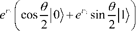
A geometrical representation of the state of a single qubit is provided by the Bloch sphere. It is often used to illustrate the effect of single qubit operations, which are elementary in quantum computing. Unfortunately, there is no equivalent representation for multiple qubits. The Bloch sphere representation of a qubit reads as
follows: | ^ ) =
. It is obtained from Eq. (0) by rewriting the complex
numbers a , a in polar coordinates, a = re 1 and a = se 1 with r , sH,^ gR and r , s - 0 , and a suitable choice of the parameters ф = 5 — ^ and 6 = 2 arccos r . It is a property of measurement that global phase factors like e 1 can be ignored. Then, a single qubit state | ^ ) can be visualized as a point
( cos ф sin 6 , sin ф sin 6 , cos 6 ) on the unit sphere in R3 as it is illustrated in Fig. 2.
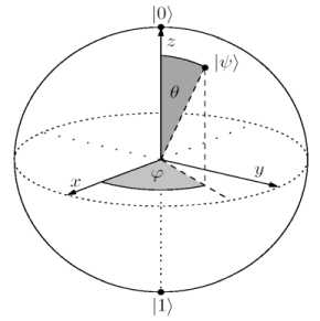
Figure 2. Bloch sphere
The x -, y - and z -axis are defined by the states ^ V2 (| 0^ +11) ) ,1/ V2 (| 0^ + 1| 1 ) and 10) .
Multiple qubits
A quantum register is a quantum mechanical system composed if several quantum bits. Considering a system of n qubits, its state space is the 2 n -dimensional Hilbert space TY( n ) : = C2 n . Similar to the 1-qubit case, the computational basis states of TY( n ) , labeled as k = \kn 4... k0 }, with k g { 0,1 } , compare to the 2 n possible states of a classical n -bit register. Here, k ... k is the binary representation of k , where k is associated with the i -th qubit. In the case where the system I in a computational basis state each qubit has a definite value, either 0 or 1 . Note that within this thesis the qubits are counted starting with 0 from the rightmost position in the ket vector (the least significant qubit), as is usual in computer science.
Any linear combination or superposition of the basis vectors is an allowed state of the system ( superposition principle ). Thus, the general (superposition) state of an n -0qubit register can be written as 2 n -1
I ^ = E aW , a k g C,0 < k < 2 n — 1. Because of the normalization condition of state vectors it is k =0
^ 2 - 1 |a P = 1. The probability for the quantum register being in state | k ) (measurement result « k») is | a |2. By convention the 2 n basis states are identified with the standard basis vectors:
C 00
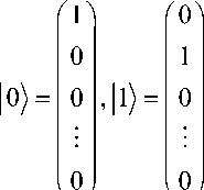
, ... ,
.
V 1 7
Mathematically, the extension from one to many qubits or the union of two or more quantum registers to a larger register is made by means of the tensor product ® :
Postulate 2. The state space of a composite system is the tensor product of the state spaces of the component systems. Let Wa) be the state of system A with state space T-^ and | w) the state of system B with state space 'HB . Then, the Hilbert space of the bipartite system AB is "H^ = TY^ ®'HB and the joint state of the total system is | w ® Wb } .
Moreover, if {| v J is an ON-basis for HA and {| ^ b} is an ON-basis for ?iB , then {I v A ' Ав } is an ON-basis for . In accordance with the tensor product of vector spaces, the dimension of is the product of the dimension of and . Therefore, the state space of a quantum register increases exponentially with the number of qubits. Abbreviated notions for the tensor product W ) ® ф of two arbitrary states W ) ® ф and ф are I w)k ) - W^ -M.
As an example, consider a system of two qubits A and B . The computational basis states (| 00), 101), |10), 111} ) for system AB results for the basis states of A and B (| 0), 11) ) by tensor multiplication: | x1x 0) = | xx ) ® | x 0), V( x 0, xx )e{ 0,1 } 2.
In multiple qubit systems there are state which cannot be expressed as a tensor product of states of its single qubit components. This property is referred to as entanglement or nonseparability . Let Wab^ be a bipartite state. If there are nay two states | ф 5) in T"^ and | ф ) in ?4 , such that Wab ) = | Ф ) ® | Ф ), the state is called separable (or unentangled); otherwise it is entangled (or unseparable). The following examples for entangled states of a two qubit system are known as the Bell or EPR states (due to Einstein, Podolsky and Rosen):
I Ф *>:= (100 + 1 "> ) • VV - (1 00 "I") ) •
I W := (I»1) + 110 ) , WV := (101> "110> ) •
When performing a measurement on a subsystem of a composite system with entangled state, another way of thinking about entanglement becomes noticeable. How entanglement is characterized by measurement is described in detail below.
Roughly speaking, quantum computation means just transforming a state of a given quantum system into another state, usually followed by a measurement. Physicists call this state transformation a (time) evolution of the quantum system, which can be mathematically represented by a unitary operator.
Remark. The matrix representation U of a linear operator is unitary (and therefore the operator itself), if UU = I, where U' =(UT )* is the complex conjugate transpose of the U matrix and I is the identity operator.
Postulate 3. The evolution of a closed physical system in a time interval [ t0, tx ] , t 0< tx is described by a unitary operator U = ( t0, tx ) which depends only on t0 and tx . Let | w) denote the state of the system at time t , then it is | W 1 ^ = U ( t 0, t i )| W^ ) .
A unitary transformation on n qubit, and thus a vector in H( n ) , is a unitary 2 n x 2 n matrix. The set of all unitary matrices of same size is a group in the algebraic sense with the matrix, multiplication as group operation. In particular, it follows:
Theorem 1. If U and V are two unitary matrices (of suitable dimension), then UV unitary as well.
Note that there are infinitely many unitary matrices of a fixed size.
Geometrically, unitary transformations preserve inner products between vectors and with it he length of vectors and the angles between vectors. They are imaginable as rotations of the vector space. Moreover, unitary operators are bijective and therefore reversible.
Following the nomenclature of electrical circuits which consist of wires and logic gates, unitary transformations are called quantum gates . May classical gates the most important quantum gates have a certain graphical representation.
A general quantum gate U operating on n qubits is illustrated in Fig. 3 (a). The short wires correspond to the incoming (left) and outgoing qubits (right). Usually, the bottom-most wire corresponds to the least significant qubit (qubit 0). Suppose U is a product of unitary transformations U and U , then an equivalents schematic symbol notation, or quantum circuit respectively, is depicted in Fig. 3 (b). Note the different
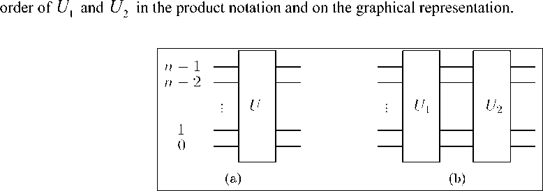
Figure 3. (a) A general n-qubit gate, denoted U. The qubits are counted from bottom (0) to top (n – 1); (b) Quantum circuit implementing U = UUX by means of Ux and U^ . (Time and control flow in the quantum circuit model goes from left to right)
Single qubit gates
A single qubit gate is identified by a unitary 2 x 2 matrix. Some important quantum gates are defined by the so-called Pauli matrices, denoted X,Y andZ :
X =
-г
( 1 Z =
1°
0 "
-1?
Their graphical representation, including the action on an arbitrary single qubit state, is shown in Fig. 4. The X -gate is equivalent to quantum NOT . Alternative symbols are a box labeled with NOT and the Ф symbol.
a | 0) + в 1 — X— в °) + a I1)
a | °) + в О — 0--г в °) + m 10
a ° + в о z a °) - в о
Figure 4. The Pauli matrices
By exponentiation of the Pauli matrices further unitary matrices emerge: calculating the matrix exponentials
e~г ^
U
, for
U
e
{
X
,
Y
,
Z
}
and
°
Bloch sphere. From the resulting matrices the following rotation operators R x , R y and R z can be easily derived
(using cos ( v ) = cos ( - V ) and sin ( - V ) = - sin ( v ) ):
R , ( ф ) =
r cos ф j sin ф
г sin ф8 cos ф ,
R y ( ф ) =
' cos ф v- sin ф
sin ф A n / а Г е - ф 0 ^ cos ф J , z ( ф ) =[ 0 e ф ?
According to this definition a gate R [ ф ] , u e { x , y , z } , is a rotation by 2 ф about the u -axis. In literature, R x , R y and R z are usually defined in a way that they perform rotations by ф (by inserting a factor of % ).
The corresponding schematic gate symbols are shown in Fig. 5.
|
— |
R , [ ф ] |
- — |
R [ ф ] |
— — |
Rz [ ф ] |
— |
Figure 5. Symbol of the single-qubit gates R x , R y and R z .
An arbitrary unitary operator on a single qubit can be written in different ways as a product of rotation matrices together with an overall phase shift factor. One way is provided by the following theorem:
Theorem 2 (X-Y decomposition of rotations). Let U be a unitary single qubit operator. Then a^^V eR exist such that U = e aRx ( ф ) R ( 0 ) Rx ( v ) .
In particular, each R z operator can be written as a product of R x and R y rotations Moreover, there is also an analogous Z - Y decomposition, where in Theorem 2 R x is substitutes by R z . Occasionally, such a general one-qubit unitary operator is denoted U 2 ( a , 0 , ф , V ) .
R z gates can also be designated as phase gates . This becomes clear when writing them in the
form Rz ( ф ) = e ф
0 8
e 2ф |
. Applied to a single qubit state the diagonal coefficient e12ф
becomes a rela-
tive phase factor regarding the 1 amplitude of the state. Because of a peculiarity of quantum measurements the global phase factor is unimportant and can be ignored. The factor 2 in the exponent can be eliminated by
defining PH ( ф ) =
Г 1
о A
. Up to a global phase factor this class f gates is equivalent to R z . Besides this
definition, the following gate is sometimes referred to as the phase gate:
S = PH ( я/ 2 ) =
Г 1
0"
г ?
The square root of gate S is gate T , the so-called я /8 gate:
T = PH (я) 4 ) =
0 8
I як
Remark. The equivalent R z -gate has diagonal coefficients e ± .
Example: Rotation matrices for SU (2). The fundamental SU (2) rotations generated by the Pauli matrices a,a and a are defined as follows: xy z ix
R , ( 0 ) = e ’
Г 0 . .0
cos
. . 00
isincos
I 2 2
■ ay 0
R, ( ° ) = e 2
r cos— sin—
2 2 R z ( 0 ) = e
. 00
- sin—cos —
I 2 2
i e2
For a general rotation, defined by the unit vector a and the angle в , we get
. aов
r. (в)=e"2"
, в в
I cos + i ( a - о ) sin
The effect of conjugating Ra by o x is the reversal of the sign of the rotation angle в iff a is perpendicular to the x -axis: oxRa (д}ох = Ra ( — в ) = R J ( в ) ^ a - ux = 0 .
Rotations about any single axis are additive: Ra ( в ) Ra ( в ) = Ra ( в + в ) .
A general SU ( 2 ) rotation G can be parametrized using the Euler angles ( а, в, у ) :
G = R , ( a ) R , ( в ) R z ( Y ) .
Another important single qubit gate is the Hadamard gate (H):
H = -T=

It maps |0) to 1/42 (| 0) + |1) ) and 1 to 1/V2(| 0) — |1) ) . Furthermore, it is H 2 = I .
In order to be applicable to an n -qubit quantum register with a 2 n -dimensional state vector, quantum
gates operating on less than n qubits have to be adapted to higher dimensions. For example, let U =
V c
b ' d J
be an arbitrary single qubit gate applied to qubit q ( 0 < q < n ) of an n -qubit register. Then the entire n -qubit
transformation, here denoted with ( ), can be written as a tensor product in the form:
U = I ® ... ® I ® U ® I ® ... ® I .
n — ( q + 1 )
q
What was intuitively clear is now confirmed: an empty wire in the graphical representation of quantum gates can be identified with the identity matrix. The matrix U consists of 2 n ( q + 1 ) major «blocks» on the diagonal, where each block contains 2 q matrices U which are diagonally arranged and shifted by one position.
The structure of U with n = 4 and q = 1 is illustrated in Fig. 6.
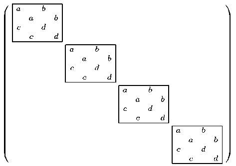
Figure 6. U consists with n=4 and q=1, of four major blocks on the diagonal, where each block contains the matrix U twice. (Within one block the structure of the 2 x 2 matrices is «broken open» and the matrices overlap each other)
Calculating the new quantum state requires 2n-1 matrix-vector-multiplications (each block, each submatrix) of the 2 x 2 matrix U. It is easy to see that the costs of simulating quantum circuits on convectional computers grow exponentially with the number of qubits. In the same way as U is a composition of I gates and U, other transformations can be built by tensor multiplication from single qubit gates which operate in parallel on different qubits.
More generally:
Theorem 3. Let U be a unitary operator on Тб m ) and V a unitary operator on H( n ) . Then U 0 V is a ( mn )
unitary operator on .
For example, applying the Hadamard gate on each qubit of an n qubit quantum register realizes the unitary transformationH®... 0 I = H0n. But there are also multiple qubit gates which cannot be decomposed n times into a tensor product of single qubit transformations, i.e., they are unseparable. This, of course, relates to entanglement of quantum states, as entangles states can only be generated by using unseparable gates.
The controlled- NOT gate, also referred to as CNOT , operates on two qubits, a control qubit and a target qubit . The action of the CNOT is as follows: it flips the target qubit if the control qubit is set to |1) and leaves it unchanged otherwise. Suppose two qubits ct are given where the first qubit it is target qubit and the second is the control qubit. Then, the effect of CNOT on the computational basis states is given by | C 1 t ) ^ | c ) 1 1 ® c ) , with c, t e{0,1} . Its matrix representational and gate symbol is shown in Fig. 7.
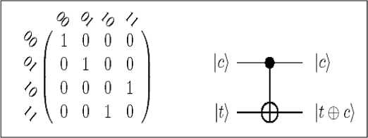
Figure 7. The CNOT gate operates on two qubits: the solid circle indicates the control qubit and the symbol ® indicates the target qubit. (The bit tuples labeling the matrix rows and columns indicate the order of basis states)
It is easy to prove that the CNOT cannot be decomposed into a tensor product of two single qubit transformations. In a similar way the ( C * NOT ) gate is defined on k + 1 qubits. It flips the target-qubit if the k control-qubits are 1. For k = 2 this gate is called a Toffoli gate or CCNOT .
It acts on the computational basis states as follows: \a, b, c} ^ | a , b, c Ф ab) for a, b, c e { 0,1 } , where a and b denotes the two control qubits and c the target qubit. Essentially, by preparing qubit c to 1 the outgoing target qubit becomes — ( ab ) . Another useful 2-qubit operation is SWAP which interchanges the states of the two input qubits: | a , b ) = | b , a^ . It can be implemented as a sequence of tree CNOT s. Its schematic symbol and decomposition in CNOT gates is shown in Fig. 8.
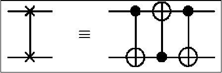
Figure 8. The SWAP gate and the equivalent circuit using CNOT gates. (The matrix SWAP is obtained by multiplication of the corresponding CNOT matrices)
More generally, let U be an m -qubit unitary operator. Then, a controlled operation C k ( U ) on k + m qubits acts on the m target qubits like the U- gate, oriented all k control qubits are 1. Otherwise it has no effect. For example, controlled phase gates with control qubit 1 and target qubit 0 are given by
( 1 0 0 0 ^
|
0 |
1 |
0 |
0 |
|
|
CPH ( ф ) = |
0 |
0 |
1 |
0 |
|
1 0 |
0 |
0 |
г ф e ) |
Similar to single-qubit gates, controlled quantum gates have to be adapted to higher dimensions, if required by the Hilbert-space. Regarding a controlled operation Ck ( U ) with single-qubit gate U , the number of matrix-vector-multiplications of U for calculating the new quantum state is reduced to 2 n - 1 - k . In that case, all diagonal coefficients, assigned to basis states which do not meet the control conditions, are set to 1, as exemplified by Fig. 9.
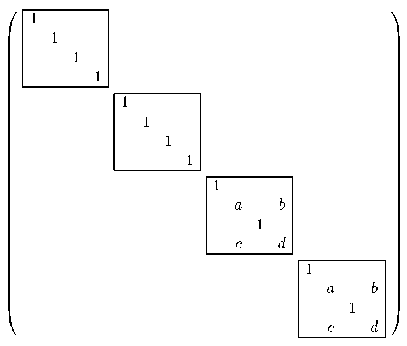
Figure 9. Controlled-U transformation with control qubits {0, 3} and target qubit 1 on a 4-qubit quantum computer. To calculate the new quantum state, only two multiplications of U with the corresponding sub vector of the current state vector are required
A gate or a set of gates is defined to be universal for classical computing, if any arbitrary gate or function can be computed requiring only those gates. Since the NAND gate is universal in classical computing and has a quantum equivalent provided by the Toffoli or CCNOT gate, the set of all quantum circuits comprises all classical circuits. However, this is only a small subset. In contrast to the discrete space of all classical operations the set of quantum operations is continuous. Therefore, the concept of universality for a discrete set a quantum gates rests on «good approximations» of arbitrary unitary operations.
In this context it is quite helpful that the sufficiently strong causality principle — similar causes have similar effects — applies also to quantum circuits, that is, small changes or errors in a single unitary operation or a gate sequence cause only small changes in the outcome of the circuit. Specifically, considering a computation where several quantum gates with a common bounded error are applied to an initial state | ^ ) , the accumulated error in the resulting state grows linearly with the length of the circuit. This motivates the following definition :
Let U and V be unitary operators acting on a Hilbert space n . V is called an approximation of U with error 6, if 6 = max I ^
||(U - V) | ^||, with | ^ g ?in, ||| ^)|| = 1. A set of quantum gates is called universal, if any unitary transformation can be approximated to arbitrary accuracy by a quantum circuit consisting of the gates from that set.
The following two theorems comprise the most important results about the universality of quantum gates and the approximation of quantum circuits.
Theorem 4 (Universality of single qubit and CNOT gates). An arbitrary unitary operation U on n qubits ( U : Hf ^ Dn ) can be realized exactly by a quantum circuit requiring O ( n 22 2 n ) gates from the set of CNOT and single qubit gates.
Theorem 5 ( Universality with a discrete set ). The discrete gate set { H , CNOT, T } forms a universal basis for quantum computation. Moreover, let U be an arbitrary unitary operation which can be realized exactly by a quantum circuit containing m gates from the set of CNOT and single qubit gates. Then, this circuit can be approximated to an accuracy c using O ( m log c ( m /c) ) gates from the discrete gate set, where c is a constant approximately equal to 2. By adding gate S , the approximations can be done fault-tolerantly.
Unfortunately, most unitary transformations cannot be efficiently implemented from a small set of elementary gates, i.e. given a unitary transformation U on n qubit; there is no circuit of size polynomial in n approximating U .
Theorem 4 is proven by explicitly constructing a decomposition of an arbitrary unitary matrix into single qubit and CNOT gates. On the following, this construction is outlined briefly. In this context, an improvement of this construction is mentioned which was introduced by Ago et all. Here, only the idea behind their approach is described.
The construction of a decomposition can be done in two steps: first, expressing the general unitary matrix of dimension d as a product of at most d ( d - 1 )/2 two-level unitary operators , that is, matrices which act only non-trivially on two or fewer vector components, as shown in Fig. 10, and second, implementing an arbitrary two-level matrix by single qubit and CNOT gates.
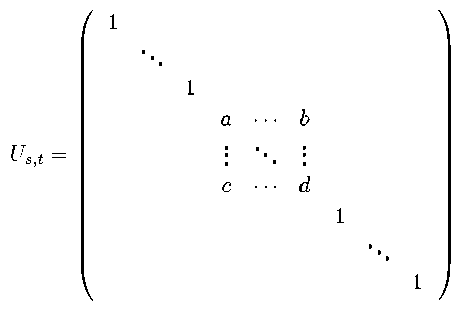
Figure 10. A two-level unitary matrix Us t with a 2 x 2 (unitary) component matrix U consisting of a, b, c, d G C (The coefficients a and b are in row s, the coefficients c and d are in row t )
The first step is also called the two-level decomposition . G. Cybenko describes this decomposition in
terms of traditional algebraic operations as a classical triangulation or QR -factorization. Since classical QR -
factorization is typically based on real valued givens rotations, which are matrices like the one in Fig. 9,
except that the component matrix is a real-valued rotation matrix U =
^ cos ф p- sin ф
sin ф cos ф ,
he calls the two-
level unitary matrices quantum givens operations . Alternatively it can be explained by means of Gray code sequences .
Thus, the entire implementation of an arbitrary unitary matrix uses O ( n 2 2 2 n ) singles qubit and CNOT gates. Aho and Svore present a decomposition algorithm with an improved two-level decomposition phase using a technique, which they call Palindrome Transformation.
Remark. They call the process that generates for an arbitrary unitary matrix an exact decomposition a quantum circuit compilation .
The idea behind this technique is, to find an optimal ordering of two-level operations in the first phase, such that the ordering of the palindromic subcircuits of self-inverting gates, resulting from the second phase, leads to a maximal amount of cancellations of the self-inverting gates: A palindromic subcircuit A is a gate sequence of the form A A ...A VA ...A A . Two successive palindromic subsequences A and B can have a subsequence of self-inverting gates in common, like ... Aj^Aj ••• AAA A ••• AjBj+i--, with Bx = A ••• Bj = A which can be reduces to ...A B....
It is shown that the Palindromic Optimization Algorithm (POA) achieves a large benefit, resulting in significantly smaller decompositions than those obtained by the conventional method. However, even for small numbers of qubits, the resulting quantum circuits are still large. It is unknown, whether there exist more efficient decomposition algorithms. Therefore, other approached might be necessary to find even shorter decompositions. Such a different approach to find optimal quantum circuits is provided by evolutionary algorithms.
In computer science an oracle is a black-box function, that is, a function whose internal working is unknown. An input for the oracle is directly processed into an output. It is said that the oracle responds on the query immediately. This implies that the costs of operating a black-box are irrelevant for complexity analysis. An oracle gate in quantum computing is usually a «variable» gate. It enables the encoding of problem instances and represents in this way the input of a quantum algorithm. Oracle gates may change from instance to instance of a given problem, while the «surrounding» quantum circuit remains unchanged. Consequently, a proper quantum circuit solving a given problem has to achieve the correct outputs (after measurement) for all oracles representing problem instances.
In certain quantum algorithms, like Grover’s or Deutsch’s, oracle gates are permutation matrices computing Boolean functions
f : { 0,1 } n ^ { 0,1 }
The transformation can be defined by the map
Uj :| x , y ) ^| x , У ® f ( x )) , |x).
f , where is
an n-qubit state, l y ^ is a single qubit state and ® indicates the
addition modulo 2. For y 0
the final state of the single qubit becomes
If (x ))
.
The oracle matrix for f inverts the output qubit, iff f yields «1» on the input qubits. In this case, the matrix swaps the amplitudes between the states differing only with respect to the output bit. As an example, Fig. 11 shows a reversible matrix implementing OR on two input bits.
|
1 |
0 |
0 |
0 |
0 |
0 |
0 |
0 |
|
0 |
1 |
0 |
0 |
0 |
0 |
0 |
0 |
|
0 |
0 |
0 |
1 |
0 |
0 |
0 |
0 |
|
0 |
0 |
1 |
0 |
0 |
0 |
0 |
0 |
|
0 |
0 |
0 |
0 |
0 |
1 |
0 |
0 |
|
0 |
0 |
0 |
0 |
1 |
0 |
0 |
0 |
|
0 |
0 |
0 |
0 |
0 |
0 |
0 |
1 |
|
0 |
0 |
0 |
0 |
0 |
0 |
1 |
0 |
Figure 11. Example for an oracle matrix, implementing the OR function of two inputs. The right-most qubit is flipped, if at least one of the two other qubits is «1»
The symbol representation of an oracle gate is usually just an appropriately labeled box, covering all the qubits the oracle is operating on. In cases where the oracle gate corresponds to a Boolean function the target qubit with the function value may be marked by the ® symbol.
Behind every oracle gate is a particular quantum circuit calculating the output. Such a quantum circuit usually gets additional inputs and needs also additional ancillary qubits which are left out in the symbol representation of the oracle. This can be done, because the additional qubits are not needed for the remainder of the computation and using a technique called uncomputing , one can get rid of the «garbage» assigned to the ancillary qubits and put them back to the initial base state. For instance, a quantum circuit for U might have additional input qubits encoding a Boolean function f which is then calculated at the output. Since any classical circuit can be simulated efficiently (in linear time) by a quantum circuit, usually one does not need to deal with the exact implementation.
Quantum information processing is useless without readout or measurement respectively. It is the final step in quantum algorithms, since there is no other way to gain information about the quantum system than by measurement. This section deals only with the projective or von Neumann measurement in the computational basis, which is a special case of a more general quantum measurement described by measurement operators. However, all other kinds of measurements proved to be equivalent to unitary transformations, using auxiliary qubits, so-called ancillae , if necessary, followed by projective measurements.
Before explaining the effects of projective measurements on quantum systems the concept of observables is introduced. An observable M is a property of a physical system that can be measured. Mathematically M is a Hermitian (self-adjoint) operator in a Hilbert space with a spectral decomposition M = £ЛкЖ • where are the eigenvalues of M. The corresponding eigenstates i of M form an ON-basis in the vector space. Here, p := |z) (i| is the projector into the eigenstate | z).
Postulate 4. A projective measurement on a quantum system is described by an observable M . The possible outcome of a measurement of M is an eigenvalue of M . After the measurement, the quantum state is an eigenstate of M corresponding to the measured eigenvalue. If the quantum state of the system just before the measurement is | ^ ), then the probability of getting result X(. is given by Pr ( i ) = || p(. | ^ || = ^ | p | ^ .
If the outcome is , the normalized post-measurement state becomes
P W
VPrco
. A projective measurement
in the computational basis {| k^} implies the use of projectors p = | k^k | to perform the projective meas- urement. For measurements in the standard basis the numerical outcomes are identified with «i». In this case, a superposition state prior to the measurement collapses with the measurement to i .
Furthermore, it is not important to known the eigenvalues X. (and thus M) , since probabilities Pr ( i ) and post-measurement states do not depend on their numerical values. In the following, the term «measure-ment» always refers to projective measurements in the computational basis.
A partial measurement of a single qubit q in an n -qubit register with outcome « i » is a projection into the subspace, spanned by all computational basis vectors with q = i . The probability Pr ( i ) of measuring a single qubit with result « i » is the sum of the probabilities for all basis states with q = i and the postmeasurement state is just the superposition of these basis states, re-normalized by the factor 1/^Pr? ( i ) . For example, measuring the first (right-most) qubit of | ^ ) = a 100) + a |o1+ a |io)+ a |11, with a0 , a , a ,, a e and | a 0|2 + a Г + l a Г + l a Г = 1, gives «1» with probability | a P + | a Г, leaving the post-measurement state | ^ = 1/^ O F+l a F ( a 1 01) + a 1 11) ) • The projectors are just P = I ® | i^i |.
It can be proved that multiple qubit measurements can be treated as a serried of single qubit measurements. Note that quantum measurements are irreversible operators, though it is usual to call these operators measurement gates . In this thesis a single qubit measurement is assigned the schematic symbol illustrated in Fig. 12.
M
-
Figure 12. Circuit symbol for a single qubit measurement
The quantum effect of entangled states was already discussed. Measurements provide another equivalent way to define entanglement. A multiple qubit quantum state is not entangles if the measurement of one single qubit has no effect on any other single qubit measurement.
Consider the entangled Bell state | ^ +) = 1/V2 (| 00) +|11) ) . Provided the second qubit has not been measured before, the probability of measuring the first qubit to be 0 is 1 2, and vice versa. If a measurement is performed either on the first or the second qubit, the measurement of the other qubit in each case gives the same result. That is, the measurement of one qubit has an effect on the measurement of the other – the measurement outcomes are correlated.
An important principle about measurement in the context of quantum circuits is discussed in the following section.
The quantum circuit model of computation is analogous to the classical circuit model. A classical circuit is made of gates computing Boolean functions and wires that connect gates. A quantum circuit has nearly the same structure, but with some restrictions.
Remark. Formally, it can be described by a (acyclic) directed graph whose vertices represent the gates and whose directed arcs represent wires.
Of course, gates in quantum circuits are quantum gates. Their graphical representation is already described. Wires, symbolized by horizontal lines, connect quantum gates and indicate input and output of a quantum circuit. Each wire represents a certain qubit. However, wires generally do not correspond to physical wires, but refer instead to a «time line». The quantum circuit fixes the chronological order of unitary transformations (plus some measurements), which are applied successively to an initialized quantum state. If not stated otherwise the input state of an n -qubit quantum circuit is the computational basis state
1 0^0 n = 1 0) ®- --® 1 0^ . By convention a quantum circuit has to be read from left to right. The simplest quantum circuit it is single quantum gate. However, to implement this gate, it usually has to be decomposed into a sequence of elementary gates.
The following rules specify the restriction of quantum circuits compared with classical circuits and define allowed connections of quantum gates in the common quantum circuit model:
|
1. |
Only acyclic circuits are valid quantum circuits, i.e. loops are not allowed. A quantum gate which into be applied repeatedly has to be wired as many times in the quantum circuit. |
|
2. |
Also, wire crossings are not allowed since arbitrary qubit permutations can be realized by SWAP operations. |
|
3. |
As a result of the reversibility of operations in quantum circuit it is not allowed to perform the FANIN operation, which joins several wires to a single wire containing the bitwise OR of the inputs. |
|
4. |
Moreover, the number of input and output wires or qubits respectively is exactly the same. |
|
5. |
In contrast to classical circuits, it is not possible to split a wire into two or more identical wires, which means, the FANOUT operation is not allowed. This corresponds to the following theorem. |
Theorem 6 (No-cloning theorem). It is not possible to make a copy of an unknown quantum state.
Even thought (universal) cloning is not possible, classical information can be copied with perfect fidelity, as any particular pair of orthogonal states can be cloned perfectly.
In the following, the main aspects of quantum circuits are summarized, beginning with a working definition of a quantum circuit and continued with explanations on inputs and outputs of quantum circuits.
A quantum circuit is a quantum computational model operating on a finite number of qubits. A quantum circuit on n qubits is a unitary operation on ?/ n ) which can be represented by a finite concatenation of quantum gates. In particle, the unitary operation is to be composed of elements from a (small) finite set of quantum gates which form a universal basis for quantum computation. Since discrete, universal gate sets realize any unitary operation with arbitrary accuracy (Theorems 4 and 5), this restriction (also important in the context of circuit evolution) does not limit the set of computable functions. A quantum circuit can get its input in two ways: (i) by the initial quantum state (the state of the qubits); or (ii) by input gates (or oracle gates), that is, unitary operations which depend on the input. The first approach is more intuitive and corresponds to the way classical circuits obtain their input. However, encoding inputs may lead to quantum systems with several qubits. Since costs for circuit evaluations on convectional computers increase exponentially with the number of qubits. Large numbers must be avoided. This is possible using the second approach.
Oracle or input gates usually substitute much larger quantum circuits and hide qubits necessary to encode further problem inputs and ancillary qubits. Yet, the use of oracle gates leads to a different complexity measure, if it is assumed, that the oracle performs its operation in a single time step. Using input gates does not contradict to the definition of quantum circuits given above. The input gate in merely integrated in the unitary operation and can be seen as an element of the elementary gate set.
Applying the quantum circuit means multiplying the unitary operation with the initial quantum state. The resulting vector provides the probabilities for all measurement outcomes. A measurement is necessary to obtain any information. From this the output of the quantum circuit can be inferred. How this is done is essentially convection. For instance, for a decision problem one can define a particular qubit to carry the answer. In a different way the output of the Deutsch-Jozsa algorithm (described at the end of this item) is obtained. Here, the measurement result of the entire quantum system is decisive for the outcome: One basis state encodes the answer « f is constant», all others the answer « f is balanced». Moreover, for optimization problems every quantum state may encode a certain solution. So, there are usually many ways to define the output modalities and the decision in favor of either way will affect the quantum circuit solving a given problem.
Note, it is still an open issue whether there exists other models of commutation which are more powerful than the quantum circuit model.
The final element in quantum circuits is the measurement. In circuits without explicit measurements at the end they are implicitly assumed. However, measurements can also be performed as an intermediate step in the circuit. Moreover, they allow conditional branchings in quantum circuits. The advantage of intermediate measurements is that they tend to make quantum circuits more «readable» and interpretable, when they are used in a clever and effective way.
In case of a single-qubit intermediate measurement, depend on the measurement result «0» or «1» one of two quantum subcircuits is applied and describes now the continued evolution of the quantum system. Multiple-qubit intermediate measurements are composed of single-qubit intermediate measurements. Therefore, it is sufficient to focus on the latter. The possibility to use intermediate measurements extends the quantum circuit model described above and requires a new definition: A quantum circuit on n qubits with intermediate measurements is a binary tree with quantum (sub)circuit on n qubits as nodes. In addition, all inner nodes of the tree are labeled with a single-qubit measurement (the qubit it acts on). By definition the left subtree corresponds to measurement outcome «1», the right to measurement outcome «0».
Applying such a circuit means evaluating a path from the root to a leaf: The quantum circuit in the root is applied to initial quantum states. Each application of a quantum circuit belonging to an inner node is followed by a single qubit measurement which determines the next subtree and the new quantum state the subcircuit is applied to.
According to the quantum principle of deferred measurement , «measurements can always be moved from an intermediate stage of a quantum circuit to the end of the circuit». Of course, such a shift has to be compensated by some other changes in the quantum circuit. The transfer of a quantum circuit with intermediate measurements to a quantum circuit without them might lead to a much larger quantum circuit (in the number of elementary quantum gates).
Note that this circuit model with intermediate measurements seems to be different to the circuit model (with intermediate measurements) roughly described by Nielsen and Chuang. Moreover, the quantum circuit models with and without intermediated measurements are computationally equivalent, but it is not quite clear how the circuit size of a quantum circuit with intermediate measurements is related to the circuit size of its equivalent circuit without intermediate measurements.
Mutually unbiased computational bases.
Measurements in a special class of bases, i.e., mutually unbiased bases, not only form a minimal set but also provided the optimal way of determining a quantum state. Mutually unbiased measurements (MUB) corresponds to measurements that are as different as they can be so that each measurement gives as much new information as one can obtain from the system under consideration. In other words MUB operators are maximally noncommuting among themselves. If the result of one MUB can be predicted with certainty then all possible outcomes of every other measurement, unbiased to the previous one are equally likely. The MUB observables can provided an explicit consideration as tensor product of the Pauli matrices for dimension d = 2 m .
Remark . When d = 2 the mutually unbiased operators are the three Pauli matrices, but unfortunately this observation cannot be generalized in a straightforward way to higher dimension. In addition to the obvious importance of MUB in the context of quantum state determination and foundations of quantum mechanics and before continuing it is useful to provide a formal definition of MUB.
Definition : Let Bx = {| ф^ ,...,| фф ^}
and B 2 = {| ^V", Wd )}
be two orthonormal bases in the d -
dimensional state space. They said to be mutually unbiased bases (MUB) if and only if (iff)

1 f ; ,
= —j= , for every i, j = 1, d
..., d . A set { B1 ,..., Bm } of orthonormal bases in C d is called a set
of MUB if each pair of bases and are mutually unbiased.
Remark . The simplest example of a complete set of MUB is obtained in the case of spin- particle, where each unbiased basis consists of the normalized eigenvectors of the three Pauli matrices respectively. However, the analysis of a set of MUB corresponding to a two level quantum system does not capture one of the basic features of MUB, i.e., its importance in determining the quantum state. In the case of two level systems, the density operator has three independent parameters and almost any choice of the three measurements is sufficient to have the complete knowledge of the system. This is not true in general for any other dimension greater than two, where the existence of MUB becomes more crucial in the context of minimal number of required measurements for quantum state determination.
Remark . Ivanovic (1981, 1997) form the first time showed that for any prime dimension d , there is a set of d + 1 MUB. There is a nice symmetrical structure behind these bases, and their existence as a consequence of properties of Pauli operators on d -state quantum systems.
Example . Let Md (C) be the set of d x d complex matrices. In a natural way, the set Md (C) is a d 2 - dimensional linear space. Each matrix A in Md (C) can be also naturally considered as a d 2 - dimensional complex vector | 9A }, where the entries of the matrix A being regarded as the components of the vector] 9 ). In this way, for matrices A, B e Md (C) we can define the inner product ( A , B ^ of matrices as the inner product 9 A , , 9^ of vectors. In this case we have the following result: ^ A , B = Tr ( A t B ) .
We say the matrices A , B e Md (C) are orthogonal iff AZ, B = 0.
Example : The existence of p + 1 MUB in the space C p , for any prime p . As mentioned above, this result first shown by Ivanovic (1981, 1997), by explicitly defining the MUB, that these bases are in fact bases each consists of eigenvectors of the unitary operators Z , X , XZ,.. , XZ d -1 , where X and Z are generalizations of Pauli operators to the quantum systems with more than two states. There is a useful connection between MUB and special types of bases for the space of the square matrices. These bases consists of orthogonal unitary matrices which can be grouped in maximal classes of commuting matrices. As a result of this connection every MUB over d consists of at most d + 1 bases.
Assume that V is a unitary operator such as V | ^ } = ^ | ^ }. Then | ^ | = 1 and for every k = 1,..., d , we have
|
^k l k i> |
= |
^k |
V l P 1) |
|
|
; = |
P1 ^k |
P 2) |
||
|
i = |
к ¥ k |
P 2) |
A similar argument shows
K^t k1) I=I ^rk Ы !=•••=! (^ kd) I •
Therefore,
К ^ k I j i2 = ^,1 - j - d •
In this case according to the Definition of MUB the next theorem is follows:
Theorem: Let Bx = {| pj,•••,] pd )} be an orthonormal basis in C d. Suppose that there is a unitary operator V such that V | p ^ = в | P+i), where ^j | = 1 and | k+1) = | k ) ; i.e., V applies a cycle shift modulo a phase on the elements of the basis B . Assume that the orthonormal basis B2 ={| ^1),...,| ^d )}consists of eigenvectors of V. Then B and B are MUB
We suppose that d is a prime number, and all algebraic operations are modulo d . We consider {| 0),Ц,.. .,| d — 1} as the standard basis of C d . We define the unitary operators Xd and Zd over C d , as a natural generalization of Pauli operators ax and az as following:
., d — 1, Sj = j + ... + ( d — 1 ) .
The action of Xd ( Zd У on | ^ k ^ is as follows: Xd ( Zd У | ^ k ^ = to + k | Vkk_ .
The standard basis {| 0),Ц,...,| d — 1 } is the set of the eigenvectors of Zd . It follows that the 2 1
| = —. Therefore, we have proved the following construction.
Theorem : For any prime d, the set of the bases each consisting of the eigenvectors of
Za , Xa , XaZa , Xa(Za )2,..., X^ Z j d —1 , form a set of d + 1 MUB d , d , dd , d d , , d d ,
Consider the particular cases of this theorem.
Case 1 : d = 2. By Theorem, the eigenvectors of the operators az , ax and oxoz form a set of MUB; i.e., the following set
|
{1 0>,|1> } |
( 72 0 0+11 ] -7? 0 0 — 1 1 ]) |
(^ 0 0+ i w ^ 77 01 0) — ' 10 1} |
Case 2: d = 3. The set of the eigenvectors of the following unitary matrices form a setoff MUB n 1 Л
( 0 0 1 J
1 Л Л
( 0 10 J
л 0 0 to2
1 0 0
^ 0 to 0 J
(0 0
1 лл
100 (0 to2
2 n .
i to = e 3
2л.
We denote the finite field { 0,1,..., p — 1 } by Fp . Let to = e d be a primitive pth root of unity. Then
ZpXp = to X p Z p .
Therefore, if U' =( X p Г ( Z- Г and U 2 ' X p ) ‘ 2 ' Z- )' 2 then
UjUx = to'- - k 2 1 UU
Example : Construction of sets MUB in the space C d when d is a prime power . When d = p m , imagine the system consists of m subsystems each of dimension p . Then the total number of measurements on the whole system, viewed as performing measurement on every subsystem in their respective MUB is ( p + 1) m . These ( p + 1) m operators fall into p m + 1 maximal noncommuting classes where members of each class commute among themselves. The bases formed by eigenvectors of each such mutually noncommuting class are mutually unbiased. It should be mentioned that the operators in each maximal commuting class have the same structure as the stabilizers of additive error correcting codes.
Let a = ( k ,..., km ) and в = (^ w-Лm ) , then a , в e F^ and we denote the corresponding operator by X p ( a ) Z p ( в ) .
Definition : The Pauli group F ( p , m ) is the group of all unitary operators
U = M , 0- • ® M m , M , = ( X p ) * " ( Z p )' - ,0 < k, , t j < p- 1
on =1 = pF 0-**0 Cp (tensor product of m copies of p)p) of the form toXp (a)Zp (в),(2)
m for some integer j > 0 and vectors а, в e F , where to = exp 5
I p
Let us consider the subset P 0 ( p , m ) of P ( p , m ) of the operators in the form of Eq. (2) with j = 0.
Remark . Note that P 0 ( p , m ) is not a subgroup, but generators of subgroups of the Pauli group can always be considered ofP 0 ( p , m ) .
If the operators U and U' in P 0 ( p,m ) are represented by the vectors ( kx,...,km\£x,...,t m) and mm
( k ‘,..., k ‘ | ^ ,..., l'm ) respectively, then U and U’ are commuting iff S jj - S k'^j =0 mod p . j =1 j=1
An explicit formula for the action of a P 0 ( p , m ) operator Xp ( a ) Zp ( в ) . The standard basis of the Hilbert space TT = C p 0 • • • ® C p consists of the vectors | j1 • • -j^ , where ( j1-- -jm ) e pm. . Then
Xp ( a ) Z p ( в )| j ?" V m ) = to j1 'в1 +'"+jm^ m |( jx + a 1 )•••( jm + a m )) .
Equivalently,
U = XD (a) ZD (в) U ' = XD (a') ZD (в') L . Po( p , m) T
Example. Let pp and pp be operators in 0 . Let
U^U* • ( a , в^Ф(a, в’^ ТТЛ 1
U ^ U , i.e., v 7 v 7. We have
|
(U , U ') |
= |
Tr ( U U ') |
|
= |
f ) Tr ^ ^ ®e " b в a\ a^a + a|b + a')(b| ( aeF. beF. J |
|
|
= |
^ < ye '' b — в a {a + a | a + a') a eF . |
While a * a , then ^i + a | a + a ') = 0, for every a e F" . Thus, in this case U , U ') = 0 . If a = a' and в * в , then ( U , U^ = ^ о)' в в) a = 0. Thus operators U and U* are orthogonal.
aeF.
|
Theorem : |
Let { A ,..., A } |
be a |
set of symmetric . x m matrices over Fp |
such |
|
that det ( A |
— Ak ) * 0 , for every |
0 < j < |
k < I. Then there is a set of + 1 1 MUB on C p |
Remark . More specifically, the ( € + 1 )-bases of the above theorem are represented by the matrices ( 0 . P . ) , (1 .( A , )(I .| A , ) .
Example : d = 4. The four matrices (over F2 = { 0,1 } ), which satisfy conditions of above theorem, are
|
f 0 0 ) 1 0 0 v |
f 1 0 ) v 0 1 J |
f 0 1 ) v 1 1 J |
f 1 1 ) v 10 J |
Therefore the classes of maximal commuting operators are
|
I = |
f 1 0 ) 0 1 v 0 1 J |
f 0 1 ) X = 1 0 v 1 0 J |
f 0 — 1 ) Y = = XZ 1 1 0 J |
f 1 0 ) Z = 0 -1 v 0 — 1 J |
We represent this basis explicitly. To this end, we naturally represent each basis by a 4 x 4 matrix such that the j th row of this matrix is the components of the j th vector of the corresponding basis with respect to the standard basis {| 00), 101), 110), 11, } : the first matrix is B^ = 14, and
|
B = |
f 1 1 1 1 ) 1 — 1 — 1 1 11 — 1 — 1 V 1 — 1 1 — 1 J |
■ 2 = 2 |
f 1 i i — 1 ) 1 — г — i — 1 1 i — i 1 v 1 — i i 1 ? |
||
|
B 3 =1 32 |
f 1 1 — i i ) 1 — 1 i i 1 1 i — i v 1 — 1 — i — i v |
■ 4 = 2 |
f 1 — i 1 i ) 1е 1е 1 i — 1 i 1 i 1 — i v 1 — i — 1 — i v |
Remark . In this case, the mutually unbiasedness condition is equivalent to the condition that BB ^ = 14 , for every 0 < i < 4 , and each entry of B^ * , for 0 < i < j < 4 , has absolute value equal to ^ .
Example : The intermediate states in mutually unbiased bases . Let us consider the two mutually unbiased bases A and A ’ that contain N basis states instead of two. We define the intermediate states between these bases. The basis A is chosen as computational basis, | a 0 ),---,| aN_^) and the second basis A’ , is the Fourier transform of the computational basis:
-
1 n-iи 1
-
1 L^
a ‘/ = ^= / exp$2n ik—aa . >.
kn л/ n n=o I
These two bases are mutually unbiased, i.e.
/ \ -\ I J О -7 n
( a. a ‘/ = — exp^ 2n ik—
' n| k' NN4
This means that the distance between pairs of state from two bases is cos
( y ) = 4=
N
Remark . Having two states, it is possible to define a state which lies exactly in between the two, which means that it has same overlap with both states and it is the state closest to the two original states which has this property . The intermediate state is obtained by forming pairs of the states from two bases. They are shown in the Table 1 below.
Table 1: Possible pairs of the states from the two bases
|
Pair |
a 0 |
a 2 |
a N —1 |
|
|
a 0 |
m 00 |
m 01 |
m0, N —1 |
|
|
a 2 |
m 10 |
m 11 |
m1, N —1 |
|
|
a N —1 |
m N —1,0 |
m N —1,1 |
m N —1, N —1 |
Explicitly the intermediate state between | an } and | a ‘ } is defined in the following way

where C = 2

is the normalization constant and the phase comes from the overlap between a and | a‘ / . The index of the m-states is such that the first index always refers to the A and the second to the A — basis. Since each basis contains N state it is possible to form N2 intermediate states, simply by forming all pairs of states from the two bases.
In general the intermediate state | m ^^between two arbitrary initial states | a ) and | ^ ) is defined as
Remark. The intermediate states may be defined in completely generality for arbitrary initial states and any number of them. In this case the intermediate state is found by forming the mixture of all initial states with equal weight, the eigenstate with the large eigenvalue of this mixture corresponds to the intermediate state. Naturally these definitions are equivalent and lead to the same intermediate state.
Example : Probabilistic interpretation of the intermediate state . Considering the intermediate states leads to the following conditional probabilities
Р ( m nk\ a n ) = P ( m nk| a ‘ ) = 1 + J = F .
Notice that this definition indeed recover the formula for cosine of half the angle:

1 + cos 0
This is why the states have been named intermediate states, since they indeed lie in between the two original states.
Whereas the probability for making an error is
P ( m nk\ a q ) = P ( m nk\ a P ) = 1
N
N - 1
D
N - 1
.
It is important to notice that the intermediate states in general not are orthogonal, indeed
(mkl\ m nm^ =
CN
NN3 e exp J ^ ^ ( mn - Ik ) ? + NN3 + + exp J ^ П ( m - / ) k L + exp J ^ П ( m - / ) n
This means that the generalized intermediate states do in general not form bases as in the two dimensional case. But they can still be used as binary measurements.
Example : Information contents of the intermediate states as binary measurements . It has been shown above that in general the intermediate states m are not orthogonal, and hence they do not form bases as in the two dimensional case. It is however possible to use the corresponding projectors, mm as binary measurements. Since the intermediate states are non-orthogonal, it means the corresponding binary measurements are mutually incompatible. In other words, none of them can be measured together but they have to be measured one by one. A binary measurement has as the name indicates two possible outcomes, 0 and 1. Where the zero outcome is interpreted as “ I guess the state was not m ”, and the “1” outcome is interpreted as “ I guess the state was m ”. However, the answers are statistical, in the sense that there is a certain probability for making the wrong identification .
It should be mentioned that the N 2 intermediate states constitutes a generalized measurement namely
N -1
so called POVM. We have — У | mu ^ mmH | = 1.
Nn7=o' 1
However, we do not make use of this in what follows. The probability of making the correct identifica- tion is given by value of F and is equal to
—I. Whereas the probability of wrong identification, i.e., 22N of an error is given by p (mnk \a) ) = ^
and is equal to
1 ( 1
N - 1 ( 2

. This means that the Shannon
information amount obtained by measurement is given by
Г 1 1 Y ( 1 1 Л ( 1 1 Y
IN = log, (N) + — +log, — ++log, inter g2 ( ) 12 2VN J g212 2VN) 12 2VN J g2
1 ( 1
N - 1 ( 2
1 )
2 V N J
Электронный журнал «Системный анализ в науке и образовании» on the “1” outcomes of intermediate state measurements.
Example : Information capacity of generalized (non-orthogonal) quantum measurements and optimal detection of quantum information . Let us to use the standard measure of information developed by Shannon, the standard definition of quantum relative entropy, and von Neumann definition of quantum entropy. Consider the particular case when two quantum systems are identically prepared in different location. It is well known that composite quantum system, consisting of non-interacting parts, can possess non-local properties. In particular, a composite system can exhibit correlations, which cannot be reproduced by any theoretical model that involves only variables belonging to each subsystem separately. A typical example is a pair of spin -^ particles produced by the decay of spin-less object. Their combined state, ^^(1ОД2)-11^2)) , cannot be reduced to a direct product by any transformation of the bases pertaining to each one of the particles (see in details Appendix 3).
Remark. We consider in this example a different kind of composite system. Its parts never interacted in past. They may have been prepared in different laboratories. However, they were prepared according to the same set of instructions. Therefore, these subsystems are in the same quantum state – insofar as their internal variables are considered. For example, we may have two non-interacting spin-^particles, prepared with the same polarization.
Let us consider the particular case in which there are three possible states for the two particles: Both 2п o^o spins may be directed along the z direction, or both may be in the x - z plane, titled at — = 120 or -120 3
from the z axis. (We have chosen this particular setup because for orthonormal projectors P = ( P , P , P ) on 2
these three directions — (P + P + P ) = I and the three possible states of each particle satis fy (^i | ^2 ) (^ | ^ X^ I ^ = - “, and this is the most negative value obtainable for such a triple product).
Suppose now that an outside observer wants to determine which one of these three known preparations was actually implemented. The answer cannot be unambiguous, because the three states are not orthogonal. The observer may nevertheless assign probabilities to the various preparations. The problem thus is to design a measurement procedure, which minimizes the unavoidable uncertainty of the result. We will to determine whether more information could be means of an apparatus interacting with both particles together, then by separate measurements performed on each one of them individually. An example of a measurement of the former type – which we will call a combined measurement – is the one represented by the “entangled” operator. The results are intriguing: New measurement technique, acting on each particle separately, yields more information than any separate – particle method.
Remark . In a von Neumann measurement model, the various outcomes are associated with orthogonal projection operators P satisfying ^ P = 1 (where 1 is the unit operator), and the probability on the i -th outcome is given by ^ | P |^ . However, instead of using a set of orthogonal operators, it may be preferable – to associate the final outcome s with a more general set of non –commuting positive operators A , satisfying ^ A = 1. The probability of getting the i -th is ^| A |^ , so that this set of A forms a probabilityoperator measure (POM). According to Neimark’s theorem such a POM is physically realizable: one can extend the Hilbert space of quantum states, in which the POM is defined, in such way that there exists, in the extended space /С, a set of orthogonal projection operators satisfying ^ P = 1, and such that A = n P П , where П is the projection operator from XL to TY . The method includes the generalized measurement that mathematically is different from simple measurement, while described by non-orthogonal expanding of unity. The measurement on any physical system can be interpreted as the simple measurement on any its enlarged section. These measurements can extract more information than simple measurements.
Let us consider two-dimensional Euclid space and fixed in this space three unit vectors
2П
(ex, e^, e3 ) = e with equal angle — between them. We can define the states Ea (x) = ( ea, xea ) , a = 1,2,3. Let the probability density functions in these directions are п = П = П = ^ and define the information amount IE (x) in extracted states Ea by an a priori probability density functions {n } . Mathematically every simple measurement is orthogonal resolution of identity in with the following properties: (i) x» > 0,»gQ; (H) ^ xto = I; (iii) xtox§ = 0, for x ^ 5 . From (iii) we are received that for every » an »
Hermitian operator xo) is a projector: x 2, = xm . If { X } is a family of positive operators inTT0 n , satisfying
N
N
^ X. < I , then defining X o = I - ^ X. we have a resolution of identity in Tn . n .
j =1
j =1
Let on the physical system {Tt, Л} in any state E is produced with probability p the simple Q - measurement {xto } , and with the probability (1 - p ) is produced another simple Q - measurement {yto } . We can introduce the generalized Q - measurement as z» = Px» +(1- P) У», and the resulting probability density function can be described as following pz (») = PE (x» ) + (1- P)E (У»).
Thus, the generalized Q- measurement z = {2ю } is equal to a randomized experiment with the simple measurements. According to Neimark’s theorem the orthogonal resolution {zto } exists. Let Tt = Tt. Tt and the spaces Tt is embedded in Tt asTt ®{0} . The relation z»
Px » + ( 1 - P ) У »
x » - У » )
is the quantity orthogonal resolution of identity in .
In this case measurement xm = ~P, » = 1,2,3, is not a simple measurement but is an extremal point of the measurement space: If x = — y + — z , then y < 2x = — P ; while P is one-dimensional proiec-» » » » » »»
tor than y^ = cP ' c^ > 0.
» » »»
The equation cp + c2P + cp = I have only one solution c = c2 = c 3 = — . It is means that in the set of generalized Q - measurements exists the measurements that are the extremal points of all measurements but are not simple, i.e., non-orthogonal.
For this case we have two possibilities: (1) the trivial expanding of unity as I + 0 + 0 + ... = I ; and (2) in two dimensional space H possible only the expanding of unit as p + p = I , where p , p are one dimensional projectors on mutually orthogonal vectors hx , h 2. Let us define the angle between h and ex as a . For this case we can define the transition probabilities as following
While cos2 a + cos2
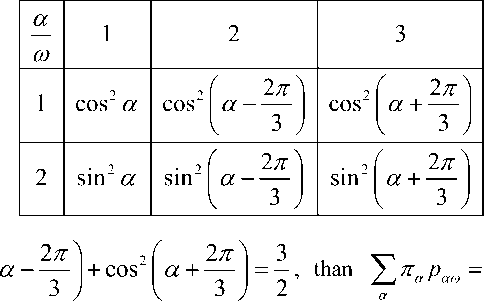
for to = 1,2 . Thus, the amount of information in extracted measurement can be defined as follows
IEa M = ln2 - 1
H ( a ) + H

-

where
H ( a ) = -
cos2 a In cos2 a + cos2 a
2n h 21
--Incos a
3 ) I
—

+ cos
. 2 n Y a +-- Incos
3 J

I П I | П I
The function H ( a ) has the following property: H ( a ) = H l a + у I = H l a — — I . From this proper-
ty we can bound the value of a as 0 < a < П and
IF (a) = ln2 — min H(a) + Ha
E a
|
a w |
1 |
2 |
3 |
|
1 |
2 — cos a 3 |
2 2( 2 п | — cos a-- 3 V 3 J |
2 2( 2п | — cos a + — 3 V 3 J |
|
2 |
2 2( 2 п I — cos a +-- 3 V 3 J |
2 — cos a 3 |
2 2( 2 п | — cos a-- 3 V 3 J |
|
3 |
2 2( 2 п I — cos a-- 3 V 3 J |
2 2( 2 п | — cos a + — 3 V 3 J |
2 — cos a 3 |
2 . .___2 ( _ ^^ I .___2 ( . . 2п I 3,
= 3,
According to the relation as cos a + cos a - + cos a + = — we have > п P„„ a aw
V 3 J x 3 J 2
(2 2 1 2 2
and I (a) = In 3 + cos2 a In — cos2 a + ; after algebraic transformations we have v J V 3 3
I3 ( a ) = ln2-- min 2 H ( a ) .
3 0< a < П
ˆ
Comparison of Eq.(2) and Eq.(4) give us I < I
There are two important measures to quantify the «costs» of a quantum program: first, the total number of quantum gates concerning a given elementary gate set and, second, the number of qubits needed to implement the circuit. To find the optimal quantum circuit both parameters have to be optimized which might be a conflicting objective. However, suppose a sufficient number of qubits is available. Then, the efficiency can also measured by the time passing from the initialization of the system state to the final measurement, which corresponds to the number of computational steps. Here, a computational step means the application of (maximally) parallel quantum gates. Fig. 13 gives an example.
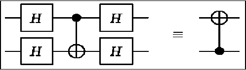
Figure 13. Quantum circuit of elementary quantum gates. The left quantum circuit consists of five elementary quantum gates
Since two Hadamard gates before and after CNOT each can be applied parallel, quantum circuit consists of three computational steps. However, the right quantum circuit is equivalent to the left circuit but consists only of a single CNOT gate.
If choosing the number of quantum gates as a measure, the simple uniform valuation model, i.e., each gate contributes the same costs, may be replaced by a more «realistic» measure, depending on a certain physical realization, which e.g. weights the costs according to the gate type. Independent of the physical implementation it might make sense, for instance, to rate controlled gates higher than single qubit gates.
Comparison between quantum algorithms which use oracle gates, so-called quantum black-box algorithms, and their corresponding classical algorithms are based on the number of accesses to input data, that is, the number of oracle calls, instead of the number of computational steps, or the number of elementary gates respectively. This complexity measure is also denoted as query complexity or decision tree complexity . Of course, a comparison of quantum and classical algorithms on the basis of oracle calls is only reasonable, of both algorithms use the same oracle.
Behind this is another computation model, the decision-tree or query model.
Strictly speaking, in the quantum version of this model (deterministic and randomized decision-trees are two other kinds) quantum circuits are studied which can be described by a unitary transformation A = U ⋅ O ⋅ U ⋅⋅⋅ O ⋅ U ⋅ O ⋅ U , where the U denote fixed, input-independent unitary transformations and the gate O an oracle call (input-dependent unitary transformation). Relevant from the viewpoint of complexity is the number of queries T .
Why investigating such a restricted model?
As it is not possible to make decisive complexity theoretical statements in more powerful computation models (this would comprise the answer to the question, whether quantum computing is more powerful than classical computing), simpler and more limited models of computation are analyzed. The hope is that understanding of such easier models will lead to a better understanding of the more complex models.
Like other promising non-standard computing approaches, quantum computing raised the hope that NP-complete problems which seem to be intractable for classical computers could be solved efficiently. Due to the merely quadratic speedup and the optimality of Grover’s quantum search algorithm, it is obvious that approaches primarily based upon (unstructured) quantum search cannot yield efficient solutions to the problems in NP, is particular to the NP-complete problems. This can be considered to be an indication that the class of NP-complete problems cannot be solved efficiently on a quantum computer. However, up to now this is neither proven nor disproven.
Complexity measures for quantum computational circuits
Apart from NP-complete problems, there are some problems, which seem to be intermediate in difficulty between P and NPC problems. This class of (decision) problems is denoted NPI (NP-incomplete) and it is NPI: = NP-NPC-P. Lander has shown that NPI is not empty, iff NP ≠ P . Thus, funding a problem in NPI would solve the most important and famous problem is computer science. For instance, the decision problem of factoring is regarded as a candidate for NPI: Given a composite integer m and l < m , decide whether m has a non-trivial factor less than l . Another problem which is still believed to be in NPI is graph isomorphism. Such problems appear to be hard classically, but they can perhaps be solved efficiently on a quantum computer, as it was shown for factoring.
Another example for a classically hard problem, but nor proven to be in NP-complete, which perhaps can be efficiently solved on quantum computers is the shortest lattice vector problem (SVP). The shortest lattice vector problem consists in finding the shortest non-trivial vector of a lattice L generated by d linear independent vectors in the vector space d . Like factoring, the difficulty of this problem ensures security in public key encryption systems (by using the inverse of this problem as a one-way function). However, the provability of Micciancio’s number theoretical conjecture would lead to SVP ∈ NPC , and this would argue against an efficient quantum solution.
From these short and unfinished reflections, it becomes convincing that quantum computing needs a separate complexity theory to understand the potentials and limitations of quantum computing compares to classical computing.
Different complexity measures for quantum circuits were already explained at the end of the last section. Another computation model is the Quantum Turing Machine (QTM) which is not explained here. While quantum circuits (like Boolean circuits) are a non-uniform computation model, because they have only constant input length, QTMs (like classical TMs) are uniform, as they work on arbitrary input lengths. As in 30
classical complexity theory, the uniform quantum complexity of computational problems is of particular interest. Therefore, analogous to uniform Boolean circuit families, uniform quantum circuit families are considered: A uniform quantum circuit family is an infinite sequence of circuit C for each input length n such that Cn can be generated by a QTM on input n (in polynomial time O ( poly ( c ( n ) ) ) where c ( n ) is the size of quantum circuit C based on a given elementary gate set. They allow a comparison of the computational power of the more abstract QTMs and the more practical (uniform) quantum circuits: It can be shown that QTMs with polynomial runtime can be simulated by uniform quantum circuits of polynomial size (with bounded error probability) and vice versa.
The following paragraph summarizes some results about quantum complexity classes (defined over QTMs) and their relation to classical complexity classes. Bernstein and Vazirani introduce quantum analogous to the classical complexity classes P and BPP EQP corresponds to P and denotes the class of problems solved error-free on a QTM in polynomial time.
Remark. BPP (probabilistic polynomial with bounded error) is the classical complexity class of decision problems that can be solved on polynomial time on a probabilistic Turing machine with bounded error probability.
BQP , the quantum version of BPP, denotes the complexity class of all computational decision problems that can be solved with bounded error probability on a QTM in polynomial time.
How EQP and BQP exactly relate to the classical complexity classes P, NP, PP, BPP and PSPACE is unknown. What is known is that
BPP c BQP c PP c PSPACE and P c EQP c BQP
Remark. PP is the classical complexity class of problems solved by randomized algorithms with unbounded error probability. PSPACE is the classical complexity class of all decision problems which can be solved on a deterministic Turing machine using polynomial space and arbitrary time.
It is still an open problem to determine which of the inclusions proper inclusions are and which are not. Especially it is not proven that BQP ^ BPP , that is, that quantum computers have capabilities beyond those of classical commuters, although there is strong evidence suggesting this.
The existing QAs described below can be naturally expressed using a black-box model. It is then useful to consider the spatiotemporal complexity of QAs from the quantum query complexity viewpoint. For example, in the case of Simon’s problem, one is given a function f : { 0,1 } n ^ { 0,1 } n and a promise that there is an s e { 0,1 } n such that f ( i ) = f ( j ) iff i = j Ф s .
The goal is to determine whether s = 0 or not. Simon’s QA yields an exponential speed-up over a classical algorithm. Simon’s QA requires an expected number of O(n) applications of f, whereas, every classical randomized algorithm for the same problem must make Q
(■)
queries 1 . The function f can be
viewed as a black-box X = ( x0,...,xN 4) of N = 2 n bits, and that an f -application can be simulated by n queries to X .
Thus, Simon’s problem fits squarely in the black-box setting, and exhibits an exponential quantum-classical separation for this promise-problem. The promise means that Simon’s problem f : {0,1}n ^ {0,1}n is partial; i.e., it is not defined on all X e {0,1}n but only on X that correspond to an X satisfying the promise.
Table 2 list the quantum complexity of various Boolean functions such as OR, AND, PARITY, and MAJORITY.
Table 2. Some quantum complexities
|
Function |
Exact |
Zero-error |
Bounded-error |
|
OR N , AND N |
N |
N |
0 ( V N ) |
|
PARITY |
N 2 |
N 2 |
N 2 |
|
MAJORITY |
0( N ) |
0( N ) |
0( N ) |
The lower bound for OR implies a lower bound for the search problem where it is desired to find an i , such that x = 1 , if such an i exists.
Thus, an exact or zero-error QSA requires N queries, in contrast to
0( VN)
queries for the bounded-
error case. On the other hand, the number of solutions is r and a solution can be found with probability 1
using O

queries. Grover discovered a QSA that can be used to compute OR with small error probability using only O (n[n ) queries. In this case of ORN, the function is total; however, the quantum speed-up is only quadratic instead of exponential.
A similar result holds for the order-finding problem, which is the core of Shor’s efficient quantum factoring algorithm. In this case, the promise is the periodicity of a certain function derived from the number to be factored.
A Boolean function is a function f : { 0,1 } n ^ { 0,1 } . Note that f is total, i.e., it is defined on all n -bit inputs. For an input x e { 0,1 } n , xt to denotes its i -th bit, so x = { xv..xn } . The expression | x | is used to denote the Hamming weight of x (its number of 1’s). A more general form of a Boolean function can be defined as f : { 0,1 } n 5 A ^ B = f ( A ) о { 0,1 } m , for some integers n, m > 0 . If S is a set of (indices of) variables, then x S denotes the input obtained by flipping the S -variables in x . The function f is symmetric if f ( x ) only depends on | x |.
Some common symmetric functions are:
-
(i) ORn ( x ) = 1 iff\x\ > 1;
-
(ii) AND n ( x ) = 1 iff \x\ = n ;
-
(iii) PARITYn ( x ) = 1 iff |x| is odd ;
-
(iv) MAJ n ( x ) = 1 iff |x | > n .
The quantum oracle model is used to formalize a query to an input x e{0,1} n as a unitary transformation O that maps |i, b, z^ to |i, b Ф x, z^ is most some m -qubit basis state, where i takes Plog n"| bits, b is one bit. The value z denotes the (m — Plog n| -1) -bit «workspace» of the quantum computer, which is not affected by the query. Applying the operator O twice is equivalent to applying the identity operator, and thus O is unitary (and reversible) as required. The mapping changes the content of the second register (| Ь ) conditioned on the value of the first register | i).
The queries are implemented using unitary transformations O in the following standard way. The transformation (O only affects the leftmost part of a basis state: it maps basis state | i , b , z^ to | i , b Ф x. , z^ . Note that the O are all equal. This generalizes the classical setting where a query inputs an i into a blackbox, which returns the bit x. . Applying O to the basis state | i , 0, z } yields | i , x. , z^ , from which the i -th bit of the input can be read. Because O has to be unitary, it is specified to map | i , 1, z } to | i ,1 - x ., z ^ . Note
1 n that a quantum computer can make queries in superposition: applying O once to the state —j= ^ | i, 0, z}
V n 1= 1
-
V n 1= 1 1
A quantum decision tree has the following form: start with an m -qubit state |0^ where every bit is 0. Since it is desired to compute a function of X , which is given as a black-box, the initial state of the network is not very important and can be disregarded. Thus, the initial state is assumed to be 10^ always. Next, apply a unitary transformation U to the state, then apply a query O , then another transformation U , etc. A T -query quantum decision tree thus, corresponds to a unitary transformation A = UTOUT_X.. .OUXOUQ . Here the U. are fixed unitary transformations, independent of the input x . The final state A 10^ depends on the input x only via the T applications of O . The output obtained by measuring the final state and outputting the rightmost bit of the observed basis state. Without loss of generality, it can be assumed that there are no intermediate measurements.
A quantum decision tree is said to compute f exactly if the output equals f ( x ) with probability 1, for all x e { 0,1 } n . The tree computes f with bounded-error if the output equals f ( x ) with probability at least ^ , for all x e { 0,1 } n .
The function QE ( f ) denotes the number of queries of an optimal quantum decision tree that computes f exactly, Q 2 ( f ) is the number of queries of an optimal quantum decision tree that computes f with bounded-error. Note that the number of queries is counted, not the complexity of the U .
Unlike the classical deterministic or randomized decision trees, the QAs are not necessarily trees anymore (the names «quantum query algorithm» or «quantum black-box algorithm» can also be used). Nevertheless, the term «quantum decision tree» is useful, because such QAs generalize classical trees in the sense that they can simulate them as described below.
Consider a T -query deterministic decision tree. It first determines which variable it will query first; then it determines the next query depending upon its history, and so on for T queries. Eventually, it outputs an output-bit depending on its total history. The basis states of the corresponding QA have the form | i , b , h , a , where i , b is the query-part, h ranges over all possible histories of the classical computation (this history includes all previous queries and their answers), and a is the rightmost qubit, which will eventually contain the output. Let U o map the initial state 1 0,0,0,0^ to | i , 0,0,0^ , and xt is the first variable that classical tree would query.
Now, the QA applies O , which turns the state into i , x , 0, 0 . Then the algorithm applies a transformation U that maps i , x ,0, 0 to j , 0, h , 0 , where h is the new history (which includes i and x ) and x is the variable that the classical tree would query given the outcome of the previous query. Then when the quantum tree applies O for the second time, it applies a transformation U that updates the workspace and determines the next query, etc. Finally, after T queries, the quantum tree sets the answer bit to 0 or 1 depending on its total history. All operations U performed here are injective mappings from basis states to basis states, hence they be extended to permutations of basis states, which are unitary transformations. Thus a T -query deterministic decision tree can be simulated by an exact a T -query quantum decision tree with the same error probability (basically because a superposition can «simulate» a probability distribution). Accordingly,
Q 2 ( f ) < R 2 ( f ) < D ( f ) < n and Q 2 ( f ) < Q e ( f ) < D ( f ) < n for all f .
If f is non-constant and symmetric, then
-
(i) D ( f ) = ( 1 - o ( 1 ) ) n ;
-
(ii) R 2 ( f ) = 0 ( n ) ;
-
(iii) q e ( f ) = ® ( n ) ;
-
(iv) Q 2 ( f ) = ® ( 7 n ( n -r ( f ) ) ) ,
where Г ( f ) = min {1 2 k - n + 1: f ^ f +1 } is quantity measure of length of the interval around Hamming weight n where f is constant. The function f flips value if the Hamming weight of the input changes from k to k + 1 (this Г ( f ) is a number that is low if f flips for inputs with Hamming weight close to n
). This can be compared with the classical bounded-error query complexity of such functions, which is 0 ( n ) . Thus, Г ( f ) characterizes the speed-up that QAs give for all total functions.
Unlike classical decision trees, a quantum decision tree algorithm can make queries in a quantum superposition, and therefore, may be intrinsically faster than any classical algorithm. The quantum decision tree model can also be referred to as the quantum black-box model.
Let Q ( f ) be the quantum decision tree complexity of f with error- bounded probability by 1. It is possible to derive a general lower bound for Q ( f ) in terms of Shannon entropy S S ( f ) defined as follows. For any f , define the entropy of f , SSh ( f ) , to be the Shannon entropy of f ( X ) , where X is taken uniformly random from A :
S Sh ( f ) = - S P y log 2 P y , where P y = Pr < R A [ f ( x ) = У ] .
yeB
For any f ,
Q (. f ) = O
SS (.f)
log n
.
In this case, the computation process can be viewed as a process of communication. To make a query, the algorithm sends the oracle | log n "| bits, which are then returned by the oracle. The first | log n "| bits specify the location of the input bit being queried and the remaining one bit allows the oracle to write down the answer.
The QA runs on J— XI x^ |^ , where X ( Y ) denotes the qubits that hold the input (intermediate
J A\xzA results of computing), respectively. It is useful to now consider the von Neumann entropy, SvN(t) (f), of the density matrix p after t -th query. If the QA computes f in T queries, at the end of computation, one expect to have a vector close to J— X | x^ | f (x)^ . For the initial (pure) state, Sv(0) (f) = 0. By using A\xzA X1 /Y
Holevo’s theorem (see [2]), one can show that SvN(T) (f) « SS* (f). Furthermore, by the subadditivity of the von Neumann entropy SvN(t+1) (f) - SvN(t) (f )| = O (log n ) for any t with 0 < t < T -1. Therefore,
T = Q
' S^h ( f ) >
V l0 g n ;
. This bound is tight.
This means one quantum query can get log n bits of information, while any classical query get no more than 1 bit of information. This power of getting O ( 1 ) bits of information from a query is not useful in computing total functions, which are functions that are defined on every string in { 0,1 } n , in the sense that each quantum query can only yield O ( 1 ) bits of information on average.
For this more general case, for any total function f ,
Q ( f ) = Q ( S '* ( f ) ) .
Kolmogorov complexity of quantum query algorithms
In the quantum query model, as in its classical counterpart, we pay for accessing the oracle, but unlike the classical case, the machine can use the power of quantum parallelism to make queries in superposition. Access to the input x g X n , where X is a finite set, is achieved by way of a query operator Ox . The query complexity of an algorithm is the number of calls to O . In quantum computing the state of computation is represented by a register R composed of three sub-registers: the query register i g { 0,1,..., n } , the answer register z gX and the work register w . We denote a register using the ket notation R = | i)|z)w , or simply i , z , w . In the quantum setting, the state of the computation is a complex combination of all possible values of the registers.
For the corresponding finite-dimensional vector space we denote the state of the computation by a vector | ^) g ?/ over the basis (| i , z , w )) . Furthermore, the state vectors are unit length for the l2norm in the quantum setting. A T - query algorithm A is specified by a ( T + 1 ) -uple ( Uo , Ux ,..., UT ) of matrices. When A is quantum, the matrices U are unitary. The computation takes place as follows.
The query operator is the unitary matrix Ox that satisfies O | i , z , w ^ = | i , z Ф xt , w } for every i , z , w , where by convention x 0 = 0 . Initially the state is set to some fixed value 10,0,0^. Then the sequence of transformations ( U o, Ox , Ux , Ox ,..., UT , Ox , UT ) is applied.
We say that the algorithm A £ -computes a function f : S ^ S ‘ for some sets S c Z n and S' , if the observation of the last bits of the work register equals f ( x ) with probability at least 1 - £ , for every £ e S . The quantum query complexity (QQC) is the minimum query complexity of quantum query algorithm that £ -compute f , where £ is a fixed positive constant no greater than .
We use a few standard results in Kolmogorov complexity and information theory. We denote the length of finite string x by x . We assume that the Turing machine’s alphabet is the same finite alphabet as the alphabet used instance of the function under consideration. Letters x , y typically represent instance; i is an index into the representation of the instance; and p , q are probability distributions. Programs are denoted P , and output of a Turing machine M on input is written M ( x ) . When there are multiple inputs, we assume that a standard encoding of tuples is used. The Kolmogorov complexity of x given y with respect to M is denoted CM ( x|y ) , and defined as follows: CM ( x|y ) = min(| P| such that M ( P, y ) = x ) , where x , y be finite strings. A set of strings is prefix-free if no string is a prefix of another in the set. The prefix-free Kolmogorov complexity of x given y with respect to M is denoted KM ( x|y ) , and defined as follows:
KM (x|y) = min(|P| such that M (P, y ) = x), where P is taken in some fixed prefix-free set. There exists a constant c > 0 such that for every finite string CT ,
K ( x | ct ) < K ( x ) + c , and K ( x ) < K ( ct ) + K ( x | ct ) + c .
Let A be a QA that for all x e S computes f , with bounded £ and at most T -queries to the input. Then there exists a constant C o such that for every x , y e S with f ( x ) ^ f ( y ) :
T > C о x —
Z
1 - 2 ( 1 - £ )
2 - ( К ( i\x , A ) + К ( iy , A )) ■
, x,* y,
Example. Grover’s QSA (see [2]). Fix n and a QA A for Grover search for instance of length n . Let z be a binary string of length log n , with K ( zA ) > log n . Let j be the integer between 0 and n - 1 whose binary expansion is z . Consider x , the all 0’s string, and let y be everywhere 0 except at position i = j + 1 , where it is 1. Then K ( i| x , A ) > log n - O ( 1 ) , and K ( i\y , A ) = O ( 1 ) .
Therefore, QQC ( QSA ) = q ( V n ) .
Thus, the minimum of Shannon entropy in the final solution output of the QA means its has minimal quantum query complexity. The interrelations in Eqs (1) and (2) between quantum query complexity and Shannon entropy are used in the solution of QA-termination problem (see below in Chapter 4). As mentioned above, the number of queries is counted, not the complexity of the U . The complexity of a quantum operator U and its interrelations with the temporal complexity of a QA is considered below.
The matrix-based approach can be efficiently realized for a small number of input qubits. The matrix approach is used above as a useful tool to illustrate complexity issues associated with QA simulation on classical computer.
-
1. Gruska J. Quantum computing. – Advanced Topics in Computer Science Series, McGraw-Hill Companies, London. – 1999.
-
2. Nielsen M.A. and Chuang I.L. Quantum computation and quantum information. – Cambridge University Press, Cambridge, Englandю – 2000.
-
3. Hirvensalo M. Quantum computing. – Natural Computing Series, Springer-Verlag, Berlinю – 2001.
-
4. Hardy Y. and Steeb W.-H. Classical and quantum computing with C++ and Java Simulations. – Birkhauser Verlag, Basel. – 2001.
-
5. Hirota O. The foundation of quantum information science: Approach to quantum computer (in Japanese). – Japan. – 2002.
-
6. Pittenberg A.O. An introduction to quantum computing and algorithms. – Progress in Computer Sciences and Applied Logic. – Vol. 19. – Birkhauser. – 1999.
-
7. Brylinski F.K. and Chen G. (Eds). Mathematics of quantum computation. – Computational Mathematics Series. – CRC Press Co. – 2002.
-
8. Lo H.-K., Popescu S. and Spiller T. (Eds). Introduction to quantum computing and information. – World Scientific Publ. Co. – 1998.
-
9. Berman G.P., Doolen G.D., Mainieri R. and Tsifrinovich V.I. Introduction to quantum computers. – World Scientific Publ. Co. – 1999.
-
10. Rieffel E. and Polak W. An introduction to quantum computing for non-physicists // ACM Computing Surveys. – 2000. – Vol. 32. – No 3. – pp. 300 – 335.
-
11. Hogg T., Mochon C., Polak W. and Rieffel E. Tools for quantum algorithms // International Journal of Modern Physics. – 1999. – Vol. C10. – No 7. – pp. 1347 – 1361.
-
12. Uesaka Y. Mathematical principle of quantum computation (in Japanese). – Corona Publ. Co. Ltd. – 2000.
-
13. Marinescu D.C. and Marinescu G.M. Approaching quantum computing. – Pearson Prentice Hall, New Jersey. – 2005.
-
14. Benenti G., Casati G. and Strini G. Principles of quantum computation and information. –Singapore: World Scientific. – Vol. I. – 2004; – Vol. II. – 2007.
-
15. Nakahara M. and Ohmi T. Quantum computing: From Linear Algebra to Physical Realizations. – Taylor & Francis. – 2008.
-
16. Stenholm S. and Suominen K.-A. Quantum approach to informatics. – Wiley- Interscience. A J. Wiley&Sons, Inc. – 2005.
-
17. Jaeger G. Quantum Information: An Overview. – N.Y.: Springer Verlag. – 2007.
-
18. McMahon D.Quantum computing explained. – Wiley- Interscience. A J. Wiley&Sons, Inc. – 2008.
References Basic definitions of quantum computing of IT students in intelligent cognitive control and robotics
- Gruska J. Quantum computing. - Advanced Topics in Computer Science Series, McGraw-Hill Companies, London. - 1999.
- Nielsen M.A. and Chuang I.L. Quantum computation and quantum information. - Cambridge University Press, Cambridge, Englandю - 2000.
- Hirvensalo M. Quantum computing. - Natural Computing Series, Springer-Verlag, Berlinю - 2001.
- Hardy Y. and Steeb W.-H. Classical and quantum computing with C and Java Simulations. - Birkhauser Verlag, Basel. - 2001.
- Hirota O. The foundation of quantum information science: Approach to quantum computer (in Japanese). - Japan. - 2002.
