Basic relations of quantum information theory. Pt 1: main definitions and properties of quantum information

Author: Ulyanov Sergey, Korenkov Vladimir, Reshetnikov Andrey, Tanaka Takayuki, Rizzotto Giovanni
Journal: Сетевое научное издание «Системный анализ в науке и образовании» @journal-sanse
Article in issue: 1, 2018.
Free access
The evolution of a quantum system can be examined from an information theory point of view. The complex vector entering the quantum evolution is considered as an information source both from the classical and the quantum level.
Quantum computing, quantum information, von neumann entropy, skew information
Short address: https://sciup.org/14123280
IDR: 14123280
Основные соотношения квантовой теории информации. Ч. 1: основные определения и свойства квантовой информации
Рассмотрена эволюция квантовой системы с точки зрения квантовой теории информации. Комплексный вектор состояния квантовой системы, описывающий квантовую эволюцию, рассматривается как источник информации как на классическом, так и на квантовом уровне.
Text of the scientific article Basic relations of quantum information theory. Pt 1: main definitions and properties of quantum information
ОСНОВНЫЕ СООТНОШЕНИЯ КВАНТОВОЙ ТЕОРИИ ИНФОРМАЦИИ. Ч. 1:
ОСНОВНЫЕ ОПРЕДЕЛЕНИЯ И СВОЙСТВА КВАНТОВОЙ ИНФОРМАЦИИ
Ульянов Сергей Викторович1, Кореньков Владимир Васильевич2, Решетников Андрей Геннадьевич3, Танака Такаюки4, Риззотто Джиовани5
1Доктор физико-математических наук, профессор;
ГБОУ ВО МО «Университет «Дубна»,
Институт системного анализа и управления;
141980, Московская обл., г. Дубна, ул. Университетская, 19;
2Доктор технических наук, профессор Института системного анализа и управления;
Директор Лаборатории информационных технологий (ЛИТ, ОИЯИ),
Объединенный институт ядерных исследований, Лаборатория информационных технологий;
141980, Московская обл., г. Дубна, ул. Жолио-Кюри, 6;
3Доктор информатики (PhD in Informatics), к.т.н., доцент;
ГБОУ ВО МО «Университет «Дубна»,
Институт системного анализа и управления;
141980, Московская обл., г. Дубна, ул. Университетская, 19;
4Доктор наук (PhD in Informatics),
Высшая школа информатики и технологии,
Университет Хокайдо;
N14, W9, Саппоро-Ши, Хокайдо, Япония;
5Доктор наук, профессор;
ST Microelectronics;
Италия, 20041 Agrate Brianza, Via C. Olivetti, 2;
Introduction: Basic concept of quantum entropy and information theory - Interrelations with measures of entanglement
Information-theoretic analysis of quantum evolution is based on the results of classical and quantum information theory. Let us consider the main results of classical/quantum information theory and its role in information analysis of quantum evolution of successful solution searching.
The most important tools and results of classical and quantum information theory Table 1 shows the most important results from classical/quantum information theory for information analysis and design of quantum evolution.
Table 1: Summary of classical and quantum information theory
|
Information theory |
|
|
Classical |
Quantum |
|
Shannon entropy : H ( X ) = - Z P x log P x x |
Von Neumann entropy : S ( p ) = -Tr ( p log p ) |
|
Distinguishability and accessible information |
|
|
Letters always distinguishable : N =1 X 1 |
Holevo-Levitin bound : H ( X : Y ) < S ( p ) - ^ P x S ( P x ) , p = 2 P x P x xx |
|
Information-theoretic relations |
|
|
Fano inequality : H ( P e ) + P e log (| X | - 1 ) > H ( XY ) |
Quantum Fano inequality : H ( F ( p , E ) ) + ( 1 - F ( p , E ) ) log ( d2 -1 ) > S ( p , E ) |
|
Mutual information : H ( X : Y ) = H ( Y ) - H ( YX ) |
Coherent information : I ( p , E ) = S ( E ( p ) ) - S ( p , E ) |
|
Data processing inequality : X ^ Y ^ Z H ( X ) > H ( X : Y ) > H ( X : Z ) |
Quantum data processing inequality : p ^E ( p ) ^ ( E 2 °E)( p ) S ( p ) > I ( p, e ) > I ( p, E оц) |
|
Noiseless channel coding |
|
|
Shannon’s theorem : nbits = H ( X ) |
Schumacher’s theorem : n bu = S ^P p qubits V x ^ |
|
Capacity of noisy channels for classical information |
|
|
Shannon’s noisy coding theorem : |
Holevo-Schumacher-Westmoreland theorem : |
||
|
C ( N ) = max H ( X : Y ) p ( x ) |
C ( 1 ) ( E ) = max { p , j P ‘ = E ( P x ) , P |
S ( p ')- E P x S ( p X ) - x _ = E P x P X x |
, |
The main problems that are investigated with these tools in information theory (that is important in an information analysis of quantum evolution) are the following:
-
• Classical, quantum and total correlations: Interrelations with entanglement measures;
-
• Accessible information and information-theoretical models of quantum measurement;
-
• Extraction of information with efficient measurements and bounds on the mutual information.
Design of quantum evolution and successful solutions is based on the same results.
Let us consider briefly these results [1-17].
Information-theoretical models of quantum system evolution and irreversible measurements
Mathematically output solutions of quantum evolution are described as quantum system entities and represented by Hilbert spaces vectors k) usually normalized Uk) = 1■ Quantum systems evolve unitarily, that is, if a system is initially in a state|k,, it becomes later state |k) after unitary operations: Uki) = |k.u Unitary operations are reversible, since UU^ = 1 and previous states can be reconstructed by: UkJ = U^ |k.. Because, кг Ui) = k |UU^ k ) = k 11k ) = 1, the operation of normalization, which soon will be interpreted as probability, is conserved. The measurement of the properties of these objects is described by a collection of operators {M m }. The quantum object will found to be in the m -th state with probability p (m) = k|M^Mm U , and after this measurement it is going to be in definite, possibly different from the starting one:
I Vs) =
-
1--- M m ------ I k ■
U U M ^ M„ I k mm
In this case m should be viewed as the measurement outcome, hence information extracted from physical system. This way information can be assigned to each state of the quantum object.
Example. In each energy state of an atom one can map four numbers or in each polarization state of a photon one can map two numbers say 0 and 1. It should be stressed here, that the measurement operators should satisfy the completeness relation: EM^Mm = 1, which results Ep(m) = Ek|M^Mm U = 1 as m mm instructed by probability theory. However this implies that k| M^Mm U ^ 1 and looking at equation
M
one understands that measurement is an irreversible operation .
Measurement process, trace and entropy Structurally, quantum mechanics has two parts: one part concerned with quantum states, the other with quantum dynamics. To find out what is going on inside a quantum system, one must perform a quantum measurement. And a partial trace operation can give the correct description of observable quantities for subsystems of a composite system: a partial trace operation consists to a projective measurement on a subsystem. The quantum operations formalism is a general tool for describing the evolution process of quantum systems, such process include unitary evolution, quantum measurement, and even more general processes.
Partial trace . The partial trace operator is the operation, which gives the description of observable quantities for subsystems of a composite system. The partial trace is defined by
Tr B (| a)(a | ®| bW\ ) = ^ЦТг (| b) b ) .
The trace is cyclic and linear.
Measurement. It is familiar that quantum mechanics describe projective measurements, “PositiveOperator-Valued Measure” (POVM), and general measurements. A projective measurement is described by a Hermitian operator, M , on the state space of the system being observed M = £ mp , where p is the m projector onto the eigenspace of M with eigenvalue m . The possible outcomes of measurement correspond to the eigenvalues, m , of the observable. Upon measuring the state |k) , the probability of getting result m is given by p (m) = (k | Pm |k).
Example: The standard (projective) quantum measurement . We start by reminding the modalities of the standard quantum measurement (of one qubit). Let us consider a qubit in the superposition state: | k = a 10) + b 11}, where 10) and 11) form an orthogonal basis, called the computational basis, and a and b , called probability amplitudes, are complex numbers such that the probabilities sum up to one: |a |2 + | b |2 = 1. The standard quantum measurement of the qubit | k ) gives either |0) with probability | a |2, or 1 with probability b 2 . This is achieved by the use of projector operators.
A projector operator P is defined by: P 2 = P , P t = P , P t = P T .
Thus a projector P is idempotent and Hermitian. Let us consider a general superposed quantum state: nn
| k = ^ c k O in the Hilbert space C n , with ^ | c j = 1 . The probability Pr ( i ) of finding the state k)
i = 1 i = 1
in one of the basis states | k ) is, after a measurement: Pr ( i ) = |P,. k )| . After the measurement, the state
' k has “collapsed” to the state k ) =
P»
7 pr(i)
n
The n projectors Pz (i = 1,2,...,n) are orthogonal: P,P = ^P,, ^P, = 1. For the case i = 0,1 we i=1
have the two 2D-projectors: Po =
r 1
V 0
0i Г 0 0i
0J M 0 1J
For which it holds: PqP, = PjP0 = 0, P 2 = Po, P 2 = P,, Po +P, = 1 . The actions of P 0 and P 1 on the basis states are, respectively:
0 Y1i
0 JI 0 ,
r 1 i
I0 J
= 10, P0l1 =
r 1 0it0i
V 0 0 J(1 ,
r0iV 0 ,
= 0
P1I0 =
r 0
V 0
0 Y 1i 1Л 0 >
r0i
V0 J
r0 0it0i r0iV 0 1JV1 J=V 1 ?
From which it follows that their action on the superposed state is, respectively:
P 0 k ) = a | 0), P 1 k ) = b |1).
The probability of finding the qubit state in the state 0 is, for example:
Pr(0) = |P0Иf = a 0)12 = a2.
After the measurement, the qubit has “collapsed” to the state:
। y -__P= y = a M = |o).
vPrro ой
Then, a lot of quantum information that encoded in qubit state is made hidden by the standard quantum measurement. As a projector is not a unitary transformation, the standard quantum measurement is not a reversible operation. This means that the hidden quantum information will never be recovered (i. e., we will not be able to get back the superposed state).
We can see that a project measurement on a subsystem is the same as a partial trace. To see it clearly, let us consider an example.
Exampe : GHZ state . In this case the GHZ state is as
I Vghz} = ^2 ( 0 A 0 B 0 C^ +1 A1 B1C of a three-qubit system ABC . Then trace one qubit (suppose of a system A ) out the three- qubit system. It has
TrA (| У GHZ ) (| У GHZ ) |) = 1 ABC + 1 ABC , where pBC = 10Д0С^0Д0С |, pBC = 11Д1С) (1д1с | • After a partial trace on system A the system of BC has a probability p = — in state pBC or in the state pBC. Obviously, the quantum measurement postulate tells us that is we perform a project measurement in basis {0),Ц} on the system A, the measurement result is in state |0) (consists to pBC) or in state |1) (consists to pBC) with a probability p = —. Consider the case the three qubit in the state | w) : | w^ = —p(| 1^0д0с^ +10Л1В0С^ + |0Л0Д1С^).
-
3 ABC ABC ABC
Let us suppose we trace out the qubit of the system A . Then we have
Tr A (| w X w l ) = I P 00 + 2 T Bc )(T Bc I, where |T Bc) = -^(|0 B 1 c ) +11 в 0 c )) is a Bell stat e.
Clearly, after a project measurement on a system A in basis { 0),Ц } , the system A has a probability 1 2
p = — in the state 11^ (consists to p 00 ) and a probability p = — in the state 10^ (consists to | T w ^ ).
Remark: Physical interpretation of quantum measurement processes . Complementarity principle tells us the microscopic world has the behavior, wave-particle duality. One cannot draw pictures of individual quantum processes. To gain information of a quantum system, one has to perform a quantum measurement. A unitary operation on a quantum system will keep the wave behavior of the system. But, a non–unitary operation will destroy the wave behavior of the system. In the quantum case, the completeness relation requires that trace of p equal to one, Tr ( p ) = 1 • We can see it consists to the quantum measurement: 1 = E p ( m ) = Z ( y | M m M m y ) • mm
A trace process can be treated as a notion that we can find out the particle in the whole space to a certain. After a trace process on a quantum system, the wave behavior disappeared completely. If the quantum 5
system is trace-preserving ( Tr ( p ) = 1 ), which means that the trace of this quantum system is unit, the probability of find out the particle is 1.
Example: Quantum dualism and quantum measurement. Consider the case of quantum measurement. When we perform a projective measurement on a quantum system, the result of the measurement is in a state with the probability p (m) = ^| M^Mm ^ . Since the state is in an orthogonal state after a projective measurement, according to the definition ^^ = ^ a, p’) of quantum system, the behavior of this system is i particle. The wave behavior disappeared. But, POVM maybe shows some wave behavior. Suppose a particle is a two-dimension {0^,Ц} quantum system. Consider a POVM containing three elements:
E i = iTT?11^11; E1 =ITT? ■ 1 w 0- i110|—^я; e = = i - Ei -
We can see that E , E and E are not orthogonal to each other. Then after a POVM, the quantum system will keep some wave behavior and appear some particle behavior.
Example: Information erasure and quantum measurement. We will assume to have a large number of bits but they will be erased individually, one by one. Landauer’s principle argues that since information erasure is a logical function, which does not have a single-valued, inverse, it must be associated with physical irreversibility and require heat dissipation. Suppose we have a quantum system, which is in an unknown state p . An information erasure process is that we prepare this system in a standard state, E : p ^ |0^0|, where p is an arbitrary state and |0^0| is a standard state. This information erasure process is non-unitary generally. If the system is in a known state, this information erasure process can be realized by a unitary operation. But in the case we have a large number of bits to erase, the information erasure operation must be irreversible. In this case information erasure will be considered as the quantum state erasure of a quantum system. Information erasure operation can be realized by a quantum projective measurement and a unitary operation: ( ’ ) M : p ^| j^j |; ( U ) U :| j)j ^ |°(0| .
First, we perform a projective measurement M . Then the quantum system will be in a known state (suppose in the state jj ) after the quantum measurement. We can perform a unitary operation U on the state | j)(j | to prepare the system in state |0^0|. Suppose we want to erase the state information of quantum system A , which is in a known state p .
We can perform a projective measurement described by projectors P . We can gain the measurement result (suppose in state j ). Then we can perform a unitary operation U to prepare the system in a state 10) . This is an information erasure process.
An information erasure operation will destroy the wave behavior completely. After an information erasure operation, the system is in state |0^0|. There is no wave behavior in this quantum system. Since the information erasure operation is physical irreversible, the wave behavior of the quantum system cannot be recurred.
Quantum operations and von Neumann entropy
The entropy of a system measures the amount of uncertainty about the system before we learn its value. It is a measure of the “amount of chaos” or of the lack of information about a system. If one has complete information, i.e., if one is concerned with a pure state, S ( p ) = 0 . A unitary operation does not change the entropy of a system because a unitary transformation does not change the eigenvalues of p .
In general, a non-unitary transformation would change the eigenvalues of p . So a non-unitary operation would change the von Neumann entropy of a quantum system.
Suppose Pj is a complete set of orthogonal projectors and p is a density operator. Then the entropy of the state p' = Z P p P t of the system after measurement is at least as great as the original entropy, i
S ( p ') - S ( p ) > 0 , with equality iff p = p . So, the uncertainty of the system increases after under the projective measurement if we never learn the result of the measurement. The entropy of the system would increase under a projective measurement. How does the entropy behave depends on the type of measurement which we perform. Projective measurement increases entropy of a quantum system. But, generalized measurements can decrease entropy of a quantum system.
Example . Consider a trace operation. The information of quantum system disappeared completely after a trace operation. So the uncertainty of the quantum system would increase. In another view, a trace process can be realized by a projective measurement if we do not know the measurement result. So a trace operation would increase the entropy of the system. Information erasure process will induce the entropy of the environment increase. Suppose a quantum system is in a state p . The von Neumann entropy of the system is: S ( p ) > 0 , where S ( p ) = 0 iff p is a pure state. After the information erasure operation, the system is in the known state 00 . The entropy of the system is zero. The entropy of the system is non-increasing. Since entropy does not decrease, the entropy of the environment must increase. To realize the information erasure process, there must be interaction between system and environment. An information erasure process has to exchange momentum-energy with environment randomly. In other view, an information erasure process can be realized by a projective measurement and a unitary operation. A unitary operation does not change the entropy of the system. The change of entropy is derived by the measurement. A measurement will induce exchange of momentum-energy between system and environment. Here, the projective measurement will decrease the entropy of a system because we have to know the result of the measurement if we want to realize the information erasure operation.
Remark . The probabilistic features of quantum states are different from that of classical thermodynamics. The difference is demonstrated by taking two totally independent facts A and B . Then the probability of both of them occurring would be: P C = P ( A ) + P ( B ) . In contrast, in quantum mechanics the wave function should be added, and by calculating the inner product probabilities are obtained. More analytically,
PQB =( VA | + (Vb |)(| V a} + VB )) = ( VA\Va} + ^B \фв )) + 2Re ^ A W in general = P(A) + P(B) + 2Re Va |Vb) * PC '
Interference
For this reason a quantum version of thermodynamics for description of quantum probability is needed. In the sequel the name “ thermodynamical probabilities” is used to distinguish the statistical mixture of several quantum states, from the quantum probabilities occurring by observation of a quantum state.
The unitary evolution of the system can be generalized by quantum operations E (p) = Z E/pE, i where Z E/E = I. Quantum operations are sometimes referred as superoperators. Quantum thermodynam-i ics just can be viewed as a transition from classical to quantum thermodynamics.
Example . Suppose an ensemble of n particles is given in equilibrium. For this ensemble says that for the i -th particle, there is a probability: p. =--- ""^e"eE i , to be in this state, where в = ( kBT ) 1 with kB
Z e - e E j j
Boltzmann’s constant and T the temperature. If the particles, where described by quantum mechanics, then if the i -th would have an eigenenergy E i , given by the solution of the Schrodinger equation H | V = E | V ), where H is the Hamiltonian of the system.
With the help of equation p. =--- -—- e eEi the density matrix p = £ p. | v) V- | can be written as:
i £ e e E i 'i
p = £ pA Vi) ( V1 = —^-pE-£ I Vt)e V | = / 1-e PH ^ Pt = —e , i £ e j i Tr (e e ) £ e j jj which is a generalization of classical thermodynamic probability pt =
£ e
e - '
Von Neumann entropy and relevant measures of quantum information theory
Willing to describe quantum information and quantum disorder, one could use quantum version of entropy, and in order to justify its mathematical definition, recall how Shannon entropy was given H ( X ) = —£ Pj log Pj , and assume that a density matrix is diagonalized by p = £ X | x^x |• Then naturally ix
A quantum entropy of p is defined as: 5 (p) =— £ X log X .
x
Translating this into the mathematical formalism, the von Neumann entropy is defined as
5 ( p )=— Tr (plog p ).
The last formula is often used for providing theoretical results and equation
A
5 (p )=—£ X, log X, x is used for calculations.
Example . Let us consider the von Neumann entropy of the density matrix
p=p (10)(0| )+(1—p) | (10)+11})«0|+01)
"\/1 — p for the quantum state | v) = pP 10) + p (| 0) +11) that is found

5 ( p ) = 5
1 — p
1— p T 2
1 — p
— X log x — X log x ,
where X = _ 1 + V1 + 2 p 2 — 2 p and X
2 L
- Г 1
2 L
— 4 1 + 2 p 2 — 2 p
are the eigenvalues of the correspond-
ing matrix.
In general case, 5 ( p ) ^ H ( p ,1 — p ) even if the same probabilities where assigned for both of them.
This shows that quantum probabilities are not expelled by quantum thermodynamics. The equality could only hold if the probabilities written in Shannon’s entropy are the eigenvalues of density matrix.
Main information measures
Following the same path as for classical information theory, in the quantum case it is straightforward to define the joint entropy , the relative entropy of p and о , the entropy of A conditional on knowing B , and the common or mutual information of A and B . Each case is correspondingly:
( i ) 5 ( A,B ) = Tr ( p AB log p AB ) ; ( ii ) S ( p|o ) = Tr ( p log p ) - Tr ( p log о ) ;
.
( iii ) S ( AB ) = S ( A,B ) - S ( B ) ; ( iv ) S ( A : B ) = S ( A ) + S ( A ) - S ( A,B ) = S ( A ) -S ( A\B )
One can see that there are a lot of similarities between Shannon’s and von Neumann’s entropies.
Example: Shannon and von Neumann measure of entropy. As measure of classical information we shall use Shannon entropy Hsh. Consider a complex vector of modulus 1 in the Hilbert space HilQ ®... ® Hi1Q , where Hil has dimension 2 for every k, written as a complex linear combination of basis vectors: | | = ^^au t |z\ ^®|i2 ^®... ® |i„ ^. Then, the Shannon Entropy of Ц with respect to the basis ii, i 2,..., in e{0,1}
{ i i) ® ... ®| i n )},,„,, E{0,1} is so defined: H Sh ( И ) =— 2 iKjf10g 0 I a - 1 i 2...j f ) , where k^- i n l |2
i i , i 2 ,..., i n e { 0,1 } '
The Von Neumann entropy is used to measure the information stored in quantum correlation. Let p = ЦЦ be the density matrix associated to state Ц and Tc { 1..... n } . Then we define: p = Tr^ я} T p , where Tr^ ирт( ... ) is the partial trace operator (see below).
The Von Neumann entropy of qubit j in Ц is defined as: S^ ( t ) = -Tr ( p T log p )
The following definitions are useful:
Remark . Measures of entropy are different from most physical quantities. In quantum mechanics one has to distinguish between observables and states . Observables (like position, momentum, etc.) are mathe-metically described by self-adjoint operators in Hilbert space. States (which generally are mixed) are characterised by a density matrix p > 0 , i.e. an Hermitian operator, with trace Tr ( p ) = 1 . The expectation value of an observable A in the state p is ^ A ^ = Tr ( pA ) . Now entropy is not an observable that means that there does not exist an operator with the property that its expectation value in some state would be its entropy. It is rather a function of state .
Si„(h) \Sr>(hk)
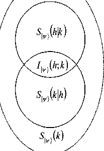
Figure 1. Wenn diagram for entropy and mutual information
Due to the Jaynes relation between the information-theoretical and physical entropy via Boltzmann’s constant, kB , one can ascribe to any quantum object a certain value of its physical entropy SC = kBH sh .
The classical limit S Cl of the expression for the entropy can be justified mathematically on coherent states. The best thing one can do is to measure the probability of finding a particle in a state with minimum uncertainty centred on the classical values, i.e. in a coherent state.
(q + ip)
Remark. In general case S'[ > S. Let, with the usual observationz := -—,— , z) = W(z) 0) be a co-ph herent state with expectation values of position, or momentum, q or p , respectively. In configuration
1 - space, |0^ is explicitly given by the wave function .— e 26 and W(z) is the unitary operator
( x 1 ( pQ — qP )
W ( z ) = e 6 with Q , P operators of position, or momentum, respectively.
We now define the classical density distribution corresponding to the density matrix p by
For every function f ( z ) there exists at most one density matrix p that p ( z ) = f ( z ) and dz
Tr p = f —(z p z) = 1. The relation Sch > S is true because, for 5(x) := {— xIn x(x > 0);0(x = 0)} due to n p concavity, s((z |p| z^)> (z|s(p) z^.
Hence: SC = d—s(p(z))> J—(z|s(p)z) = Tr(s(p)) = 8(p). П П dz
More generally, for any convex (concave) function f, Tr (f (p))<(>)[ —f (p(z)). By continuity n of p(z), SCl = S would imply s(^z p|z^)= ^z|s(p)z^ for allz , i.e. regarding the strict concavity of S(•), every | z^ must be an eigenvector of p, which is impossible.
Hence, S C > S .
Remark. The classical entropy is not invariant under every unitary transformation, i.e. we do have not
S Ch ( U pU ) = S Cl ( p ) for every U but for a restricted class only. For instance if U = W ( z 0 ) , then
SC (W (- --0 )pW h )) = J dzS «0 W (- z )W (-• 0 W (--0 W ^) 0) )= J —S (p( z + z, ))= SC (p).
П П
This argument also works for all unitary U such that UW ( z ) = W ( z ' ) times a phase factor provided that dz = dz ' (canonical transformation).
If | ^ is a pure state (unit vector), p = | V}^ |. Then p ( z ) = | ^ |z ^| , and
S Ph ( p ) = — 2 J dz l M z hl( И z Г.
Inserting for| ^ = | z 0), we obtain: SCph(p )= [ — e 'z' • | z |2 = 1 .
n
On the other hand, there exist pure states with arbitrary high classical entropy: it suffices to show that for every 8 > 0 one can find unit vectors | ^ such that ^| z ^ < 8 for all z .
For them a well-known inequality tells us that: Sdph ( p ) > — In 8 2 .
We conjecture that the states with minimal classical entropy are exactly given by the density matrices | z^z |, and consequently, S ^ ( p ) > 1 .
In order that S ^C p ) be small, Supp ( z ) must be close to one, otherwise the inequality mentioned before gives a value too large for classical entropy. Now if Supp ( z ) is exactly equal to 1, then, by continuity, there is some z 0 with p ( z 0 ) = 1 , i.e. ^ z0 p| z 0 ^ = 1 . Since || p || < 1 this implies || p || = 1 and p ( z 0 ) = | z0 ,; on the other hand, Tr ( p ) = 1 , hence p = | z0 ^z 0 | because all other eigenvalues of p must be 0.
Thus in general case S C > SC . These entropies are used below in information analysis of the quantum evolution.
The quantum conditional entropy S ( X | Y ) is defined by a natural generalization of the classical case as n
1 _1
SvN ( X I Y ) = — Tr XY [ p xy lg p xy ] , where p x Y = Jim p XY (I x ® p Y ) n
, which should be an analogue to the conditional probability p(x I y). The quantity IX is the unit matrix in the Hilbert space for X and pY = Tr[pXY] denotes a “marginal” density matrix - an analogue to the “marginal” probability Py =^ P(x, У). The above definition of S(X | Y) leads to an analogue of the classical Shannon theory x holds also for quantum entropy: SvN(X | Y) = SvN(X, Y) — SvN(Y).
The complicated expression of p XY and the fact that a limit has to be used are due to the fact that the joint density matrix ( p XY ) and the marginal matrices I X ® p Y do not commute in general. If they do commute, the whole expression gets much simpler, as discussed below. In spite of the apparent similarity between quantum SvN ( X | Y ) and classical SSh ( X | Y ) the fact that in the quantum case we deal with (density) matrices, rather than with numbers, as in the classical case, brings quite a different situation for quantum information theory and potential far exceeding the classical one.
While p ( x | y ) is a probability distribution in x (i.e., 0 < p ( x | y ) < 1 ), its quantum analogue p ( X | Y ) is not a density matrix. It is Hermitian and positive but its eigenvalues can be larger than 1 and, consequently, the conditional entropy can be negative .
This helps to explain the well-known fact that quantum entropy is non-monotonic, and it can be the case that SvN(X, Y) < SvN(Y), i.e. the quantum entropy of the entire system can be smaller than entropy of one of its subparts (what is not possible in the classical case). This happens, for example, in the case of quantum entanglement as shown in the following example.
Example. Consider the Bell state | ^ ) = -E(| 00) +111) ) of the Hilbert space H^5 = Нл ® H5 , where
H A = h B = h 2 . The density matrices p AB = | ^)( ^ |, p A , p a i b are as follows:
|
1 ) |
||
|
^ A f 10 0 1 ^ |
1 0 0 2 |
2 |
|
2 0 0000 _ |
0 0 0 |
0 |
|
p A = 1 , p A 1 B = 0 0 0 0 , and p AB = |
0 0 0 |
0 |
|
0 - |
||
|
I 2 J 1 0 0 |
1 0 0 |
1 |
|
1 2 |
2 J |
Hence: S vN ( A ) = S vN ( B ) = 1 . The density matrix is p AB = p AB (I A ® p B ) 1 (because in this case the joint and marginal matrices p AB and I A ® p B commute).
Hence, S ( AB ) = S ( B ) + S ( A | B ) = 1 - 1 = 0 because S ( A | B ) = - 1.
Unlike in classical (Shannon) information theory, quantum (von Neumann) conditional entropies can be negative when considering quantum entangled systems, a fact related to quantum non-separability, so that entanglement might be viewed as super-correlation .
Quantum mutual information I ( X : Y ) , as an analogue of the classical mutual information I ( X : Y ) is de
1 - 1 1 n
( p x ® p y ) n p XY
, and the definition implies the
fined on the base of “mutual” density matrix pX.Y = lim n ^^
standard relation: I ( X : Y) = S ( X ) - S ( XIY) = S ( X ) + S ( Y ) - S ( XY) .
This definition is reduced to the classical one for the case where p XY is a diagonal matrix.
However, not all basic equalities and inequalities of the classical information theory transfer from the classical to the quantum case. For example, in the classical case: I ( x : y ) < min[ S ( x ), S ( y )] , but in the quantum case the best upper pound possible is S ( X : Y ) < 2min[ S ( X ), S ( Y )] .
Additional basic properties of quantum von Neumann entropy are summarized below:
|
Invariance : SvN ( p ) = SvN(U*pU ) for any unitary matrix U ; |
|
if p = ^p + ^ 2 p 2, ^ + ^ 2 = 1, ^ > ^ 2 > 0 , then S vN ( p ) > ^ S vN ( p^ + X 2 S vN ( p 2 ) ;
S ( E P i- p A ® p B ) > max { e PS ( p A ) +E s ( P i- p B ) , E Pi S ( p B ) +E s ( Pip A ) } |
|
|
|
А = Т- в р , р 2 = T- А р , then S vN ( р ) < 5 vN ( р ) + 5 vN ( р 2 ) < 5 vN ( р х ® р 2 ) ; |
|
|
Lower bound : 5 vN ( р ) > - log ^ , where Х х is the largest eigenvalue of р . |
|
|
Triangle inequality : 5a - 5b < 2 5 C < 5 a + 5 B , 5 C = 1 ( 5a + 5 B ) |
Relative entropy
The classical Kullback-Leibler information admits several extensions to the quantum case. The most successful appeared the most straightforward definition due to Umegaki as:
5 (р к) = Tr (р log р)- Tr (р log с).
This entropy is an important tool in the quantum theory of noise channels. Its basic property is monotonicity ( Uhlmann inequality ). We have for any quantum operation Л :
-
5 (л р ||Л с ) < 5 ( р к ) .
This inequality can be viewed the counterpart of the Boltzmann H-theorem in statistical physics.
As such one can prove the following result:
5(р||с) > 0, 5(р||с) = 0 ^ р = с, and is known as Klein’s inequality. This inequality provides evidence of why von Neumann relative entropy is close to the notion of metric. Relative entropy satisfies also the following inequality:
-
5 ( рк ) > 11 р - с 11,
which is generalization of the similar one for Kullback-Leibler relative entropy.
Main properties of relative entropy are as following:
|
Monotonicity of relative entropy under completely positive, trace preserving maps Ф 5 ( ф ( р )IH c )) < 5 ( рк ) |
|
|
Monotonicity of relative entropy under partial trace 5 ( р А || к ) < 5 ( р ас Ик с ) |
|
|
Strong subadditivity of von Neumann entropy I and II, where I and II are equivalent
|
|
|
Joint convexity of relative entropy 5 ( х р,р‘\рк ) <х p,s ( р ' к ' ) |
|
|
Generalized (equivalent) inequality, concavity of conditional entropy |
|
S ( s Pp « ) - 5 ( s Pp, ) i! p, [ 5 ( p AB ) - S ( p B ) ] |
|
|
The entropy exchange Sex ( p , E ) for a quantum operation S ( E ( p ) ) - S ( p ) + S e, ( p , E ) > 0 |
Since these five inequalities are equivalent, we can obtain any one of them from one of the other four inequalities.
Remark . The Kullback-Leibler divergence offers an information-theoretic basis for measuring the divergence between two given distributions. Its quantum analog fails, however, to ply a corresponding role for comparing two density matrices, if the reference states are pure states. The non-additive quantum information theory inspired by nonextensive statistical mechanics is free from such a difficulty and the associated quantity, termed the quantum q -divergence, can in fact be a good information-theoretic measureof the degree of state purification. The corresponding relation between the ordinary divergence and the q -divergence is violated for the pure states, in general.
Example : Quantum Kullback-Leibler divergence . In classical information theory, a comparison of two distributions is customarily discussed by employing the Kullback-Leibler divergence. Its quantummechanical counterpart is the quantum divergence of a density matrix p with respect to a reference density matrix c , which is given by:
K[pc] = Tr [p(lnp - lnc)], where the equality holds iff p = c . However, since In c is a singular quantity if the reference state c is a pure state, this quantity turns out to be inadequate for a measuring degree of purification. The quantum q -divergence is obtained by replacing the derivative
K [ p|c ] = dXTr ( pc x )
x ^ 1- 0 ,
with the Jackson q -derivative:
Kq [ PH ] = DqTr ( PXc1-' )
X ^1-0
where D q
f (qx)-f (x) x ( q - 1)
denotes the Jackson differential operator. Than K [ p ||c ] can be defined as
Kq [p c] = , 1 Tr [pq (p'“ - c'“ )] = Tr [pq (lnq p - lnq c)] '
1 — q
The crucial difference between K [ p||c ] and K [ p||c ] is that, in marked contrast with In c , ln? c is a well-defined quantity for a pure reference state c = | k)k | . In fact, in this case, c1 q = c ( 0 < c < 1 ) , whereas ln c = ( c — I ) Z ( 1 ) , which is divergent, where I and Z ( 1 ) are the unit matrix, and the Riemann Z function, respectively.
Accordingly, equation Kq [ p||c ] = Tr i p4 ( ln? p — ln? c ) I is seen to be:
Kq [ p|lc=Ик I ]=71- (1 - kpq k)).
1 - q
The additive limit q ^ 1 cannot be taken in this equation anymore.
Particular case . Let p is also a pure state, p = | ф ф |. Then
K q [I ФФ|| к)^ |] = d F^ •
1 - q where d2S = 1 -1ф|^^| is the Fubini-Study metric in the projective Hilbert space, which may give the geometric interpretation to quantum uncertainty and correlation.
Example: Purification of Werner state. The Werner state is a state of a bipartite spin- system, i.e., two qubit, given as follows:
p w =
1 - F
+-- where H=4 (i0i) ±i 10)) ,i «*)=-к (i 00) ±i ii)) are the Bell states, and F is the fidelity with 22
respect to the reference state 7 = IT -д T - I.
Its allowed range is —F F < 1 , and pw is known to be separable iff F < — .
The quantum q -divergence of p with respect to the reference state < 7 = | T ^T | is calculated to be
K [ pw| 7-lT-)(T-l]-A (1 - F)-0 ■
1q where the zero value is realized when F = 1 or q ^ 0+. However, as already stressed, the limit q ^ 1_0 is singular and does not commute with the limit F ^ 1 0 .
Remark . The relative entropy is used as a distance; this distance is not a metric because it is not symmetric under interchange of the states. Corresponding to Shannon’s entropy, S ( p ) < log d , S ( p ) = log d O' p = — . In addition to this from definition of von Neumann entropy it follows that: S ( p ) > 0, S ( p ) = 0 о p is pure .
One can also prove that supposing some p states, with probabilities p, have support on orthogonal subspaces, then:
S (z Pipi) = H (Pi) + Z pS (pi).
Directly from this relation the joint entropy theorem can be proved, where supposing that p are probabilities, | г^ are orthogonal states for a system A , and p is an set of density matrices of another system B , then:
S (z pi. | Iх) ii 10 pi) = H (pi.) + Z PiS (pi-) .
Example: Splitting of information in a particular quantum state into classical and quantum part. Con-„ . , t i AipAA _ . , , , sider performing a general measurement on the state, A.A . , such that p = —з-------. The final state
Tr ( A i P B A t )
of subsystem B is then E AzpBA t = E РгplB . The entropy of the residual states is E ptS (pB ). The classi-ii i cal information obtained by measuring outcomes i with probabilities pz is H (p) . If the states pB have support o orthogonal subspaces, then the entropy of the final state is the sum of the residual entropy and the classical information, i.e.,
S (e p pa ) = H (p )+z pS ( Pb ).
Class cal
Quantum
It has been shown that the state p = E pzP i g can be reconstructed with arbitrary high fidelity from the
i classical measurement outcomes and the residual states iff the residual states pB are on orthogonal subspaces. We see then that the information in a quantum state may be split into a quantum and a classical part.
The entropy of tensor product p ® a is found to be S ( p ® a ) = S ( p ) + S ( a ) . Another result can be derived by Schmidt decomposition (see, in details Vol. 83).
If a composite system AB is in a pure state, it has a subsystems A and B with density matrices of equal eigenvalues, and S ( A ) = S ( B ) .
A great discrepancy between classical and quantum information theory is quantum entanglement and its measures. The tools described in above can help reveal a great discrepancy between classical and quantum information theory: entanglement .
Entanglement
In quantum mechanics two states are named entangled if they cannot be written as a tensor product of other states. For the demonstration of the above mentioned discrepancy, let for example a composite system AB be in an entangled pure state AB , then, because of entangled, in the Schmidt decomposition it should be written as the sum of more than one terms: |AB^ = E А 1^)1^) , with |I| > 1, where |i^and \гв^ are i e I orthonormal bases. The corresponding density matrix is obviously pa = AB)(AB| = E Л2/|'".,)|'в)ШШ.
-
i , j e I
As usually the density matrix of the subsystem B can be found by tracing out system A , pB=TrA (p AB) = E xixj k kA WkAX A A kA^jAB I=E2-21 гвЖ I.
-
i, j , k e I i e I
Because of assumption | I | > 1 and the fact that | i s ^are orthonormal bases and it is impossible to collect them together in a tensor product, subsystem B is not pure. Thus, according to the property: S ( p ) > 0, S ( B ) > 0 , AB is pure and S ( p ) = 0 ^ p is pure , thus S ( A , B ) = 0 and obviously by the definition
-
( iii ) S ( AB ) = S ( A,B ) - S ( B ), S ( AB ) < 0 ,
-
i .e., negative .
The last steps can be repeated backward and conclusion, which can be drawn, is that a pure composite system AB is entangled iff S ( AB ) < 0 .
Remark. In classical information theory conditional entropy only be H (XB) > 0 and that is obviously the reason why entangled states did not exit at all. This is an exclusive feature of quantum information theory. Entangled states are named after the fact S(AB) < 0 ^ S(A,B) < S(B) , which means that the ignorance about a system B can be in quantum mechanics more than the ignorance than of both A and B . This proposes some correlation between these two systems.
Example . Imagine a simple pair of quantum particles, with two possible states each 10^ and 1. Then a possible formulation of entanglement can be a state | ^ = -4= 10^ ® 10^ + -4= Ц ® Ц .
After a measurement M of the first particle for example, according to
| ^ = , m |^), Mm |^ = 1(| m ® | m)) + 0(1 - m)®(1 - m) = m ® | m,
IBM^ M„ Ы^ mm hence they collapse to state m .
This example sheds light into the quantum property, where ignorance of both particles is greater than the ignorance of one of them, since perfect knowledge about the second.
Basic properties of von Neumann entropy and Wigner-Yanase-Dyson skew entropy
The basic properties of von Neumann entropy (which can be compared to the properties of Shannon en- tropy) shown in Table 2.
Table 2. Main properties of von Neumann entropy
|
Property of von Neumann entropy |
|
|
Symmetry : S ( A , B ) = S ( B, A ) ; S ( A : B ) = S ( B : A ) |
|
|
Unitary operations preserve entropy: S ( U p U ^ ) = S ( p ) |
|
|
Subadditivity : S ( A, B ) < S ( A ) + S ( B ) |
|
|
Triangle (or Araki-Lieb ) inequality : S ( A, B ) > S ( A ) — S ( B ) |
|
|
Strict concavity of the entropy : Suppose that are probabilities p z > 0 and the corresponding density matrices p , then
S
(
z
pp.
)
|
|
|
Upper bound of a mixture of states : Suppose p = Z pz p where p z > 0 are probabili- i ties and the corresponding density matrices p. , then
S
(
p
)
|
|
on orthogonal subspaces |
|
|
Strong subadditivity : S ( A , B , C ) + S ( B ) < S ( A, B ) + S ( B, C ) , or equivalently S ( A ) + S ( B ) < S ( A, C ) + S ( B , C ) |
|
|
Conditioning reduced entropy : S ( AB , C ) < S ( AB ) |
|
|
Discarding quantum system never increase mutual information : Suppose ABC is a composite quantum system, then S ( A : B ) < S ( A : B , C ) |
|
|
0 |
Trace preserving quantum operations never increase mutual information : Suppose AB is a composite quantum system and E is a trace preserving quantum operation on system B . Let S ( A : B ) denote the mutual information between systems A and B before E applied to system B , and S ( A' : B ') the mutual information after E is applied to system B . Then S ( A : B ') < S ( A : B ) |
|
1 |
Relative entropy is jointly convex in its arguments: Let 0 < X < 1, then S ( X A + ( 1 — X ) A ,| X B + ( 1 — X ) S , ) > X S ( A ,| B , ) + ( 1 — X ) S ( A ,| B , ) |
|
2 |
The relative entropy is monotonic: S ( pA B B ) < S ( pAB | B AB ) |
Partial trace, entropy inequalities and skew-entropy
The partial trace operation described above and the strong subadditivity property of entropy in quantum information theory can be explained also in linear algebra terms. Let A be a density matrix and K any selfadjoint operator. For 0 < t < 1 let
St (A,K) = 1 Tr [At,K][A1"t,K], where [X, Y] = XY — YX stands for commutator.
This quantity is a measure of non-commutativity of A and K , and is called skew-entropy of Wigner-Yanase-Dyson (see below). This too is a concave function of A , a consequence of a more general theorem.
Theorem 1 ( Lieb): The function f ( A, B ) = Tr ( X * A‘XB 1—1 ) of positive matrices A, B is jointly concave for each matrix X and for 0 < t < 1
Using the familiar identification of L ( H ) with H ® H * , this statement can be reformulated as: the function g ( A, B ) = A t ® B 1 — t is jointly concave for 0 < t < 1 .
Another quantity of interest is the relative entropy:
S ( A\B ) = TrA ( log A — log B )
associated with a pair of density matrices A, B . If f is any convex function on the real line, then for Hermitian matrices A, B
Tr [ f (A) —f (B )] > Tr [(A — B) J"(B )].
This inequality (called Klein ’s inequality ) applied to the function f ( t ) = t log t on the positive halfline shows that for positive matrices A , B ,
If A, B are density matrices, then Tr [ ( A — B ) ] = 0 , and hence S ( AB ) > 0 . It is easy corollary of Lieb’s concavity theorem A9.1 that S ( AB ) > 0 is jointly convex in A,B .
Remark . Choose X = I in f ( A, B ) = Tr ( X * A XB^ 5 ) and differentiate this function at t = 0.
Finally, we come to the properties of entropy von Neumann S ( A ) and S ( AB ) related to partial trace . Let A , A be density matrices. It is easy to see that S ( A ) is additive over tensor product: S ( A , A ) = S ( A ) + S ( A ) . Now let A be a density matrix on H ® H2 and let A , A be its partial traces. The subadditivity of S ( A ) says that: S ( A ) < S ( A ) + S ( A ) .
This can be proved as follows. From S ( AB ) > 0 we have
0 < S ( AA ® A ) = TrA (log A — log ( A ® A )) = TrA (log A — log ( A ® I) — log (I ® A2)) = Tr ( A log A — A log A — A2 log A2) = — S (A) + S (A) + S (A)
It is obvious that S ( UAU* |UBU *) = S ( AB ) for every unitary matrix U .
Hence, from the representations
1 m — 1 1 m — 1
ФА A ) = — У W* k AW k , Ф2( A ) = — У X* k AX k , m k = 0 m k = 0
W = U®Ue...® U (n copies) , X = V ® Ve...® V (n copies),
■ f A =[ A» ] 1 < 1, j < n, is partial trace we see that
S(Ф2 „Ф, (A)|Ф2 Оф, (B)) < S(Ф, (A)|Ф1 (B)) < S(AB).
Thus we have S ( AB ) < S ( AB ) .
More general result can be proved using same techniques: if Ф is any completely positive, trace-preserved (CTP) map, then S ( ф ( A )| ф ( B ) ) < S ( AB ) .
Now consider a tensor product H ® H2 ® H3 of three Hilbert spaces. For simplicity of notation let us use the notation A for an operator on this Hilbert space, and drop the index j when we take a partial trace TrH . Thus Tr^A^ з = A2, Tr^A2 = A , etc. Using the diminish property
S ( Ф ( A )| Ф ( B ) ) < S ( AB ) with respect to the partial trace TrH?A2 3 = An we see that
S ( AK \A, ® A 2 ) < S ( ^2з| A , ® A 3 ) .
We have seen providing S ( A ) < S ( A ) + S ( A ) that
S(TT ® T2) = -S(T) + S(T) + S(T).
So the above inequality can be written as
-
- S (A,2) + S (A,) + S (A )<- S (A2,) + S (A,) + S (A,)
and on rearranging terms, we are received strong subadditivity of entropy is the following statement.
Theorem 2 (Lieb-Ruskai): Let An 3 be a density matrix on H ® H2 ® H3. Then
S (A,,,) + S (A )< S (A„) + S (A,,).
The partial trace operation described above and the strong subadditivity property of entropy in quantum information theory can be explained also in linear algebra terms.
Information-theoretic models of quantum measurements . There are two types of evolution a quantum system can be undergone: unitary ; measurement .
The first one is needed to preserve probability during evolution.
The information-theoretic interpretation of entropy is in this case as following: Entropy is the amount of knowledge one has about a system.
One is relieved by seeing that knowledge can decrease or increase by measurement, as seen by Results 1 and 2 (see below), and that is what measurement was meant to be in the first place.
Result 3 instructs that if only unitary evolutions were present in quantum theory, then no knowledge on any physical system could exist.
Thus information theory can explain why a second type of evolution is needed as following.
|
Measurement |
Entropy law of evolution |
|
1. Projective measurement |
Projective measurement can increase entropy : This is derived using strict A concavity. Let P be a projector and Q = I — P the complementary projector, then exist unitary matrices Ux , U 2 and a probability p such that for all p , PpP + Q p Q = pUP 2 + ( , - p ) и 2 pu 2 , thus s ( PpP + Q p Q ) = s ( pu , pu 2 + ( ,— p ) и 2 ри 2 ) > pS ( и , ри 2 ) + ( ,— p ) s ( и 2 ри 2 ) = ps ( р ) + ( 1 — p ) S ( р ) = S ( p ) Because of strict concavity the equality holds iff PpP + QpQ = р |
|
General measurement can decrease entropy : One can convenient by considering a qubit in state р = —10)(0 +~ K,, which is not pure thus S ( р ) > 0 , which is measured using the measurement matrices Mx = 10^ ^0 |
|
2. General measurement |
and M 2 = 0)(1 . If the result of the measurement is unknown then the state of the system afterwards is p' = MxpM ^ + M2pM2 = |0^0|, which is pure, hence 5 ( p ') = 0 < 5 ( p ) |
|
3. Unitary evolution |
Unitary evolution preserves entropy : This is already seen as von Neumann’s entropy property |
Accessible information
Some very important results derived by information theory, which will be useful for the development, concern the amount of accessible information and how data can be processed.
Accessible classical information: Fano’s inequality . Let X = f ( Y ) is some function, which is used as the best guess for X and let pe = p ( X Ф X ) be the probability that this guess is incorrect. Then an “error” random variable can be defined as following:
E = ^
1, X Ф X
0, x = X
thus H ( E ) = H ( pe ) . Of major importance, in classical information theory, is the amount of information that can be extracted from a random variable X based on the knowledge of another random variable Y .
That should be given as an upper bound for H ( XY ) and is known as Fano’s inequality :
H ( P . ) + P . log (I X | -1 ) 2 H ( XY ) .
Accessible quantum information: quantum Fano’s inequality and the Holevo bound
There exists analogous relation to above classical Fano’s inequality, in quantum information theory, named quantum Fano’s inequality :
5 ( p, E )< H ( F ( p, E )) + (1 - F ( p, E )) log ( d2 -1), where F (p, E) is the entanglement fidelity of a quantum operation defined as F (p, E) = Z Vr (pE )l2. i
E are the operation elements of E . Quantum fidelity quantifies how much entanglement between subsystems sent a quantum channel E is preserved (see measure definition of quantum fidelity below). In the above equation, the entropy exchange of the operator E upon p was introduced as 5 ( p, E ) = 5 ( R ‘, Q ‘ ) , purified by R . The prime notation is used to indicate the states after the application of E . The entropy exchange does not depend upon the way in which the initial state of subsystem Q is purified by R . This is because any two purifications of Q into RQ are related by a unitary operation on the system R , and because of von Neumann entropy property.
Remark . Quantum Fano’s inequality is proven by taking an orthonormal basis i for the system RQ , chosen so that the first state in the set |1) = | RQ ). Forming the quantities рг = it \ RQQ |i ^ , then it follows that S ( R ', Q ') < H ( p1,...,pd 2 ) , and with some algebra
H ( Pv’, Pd 2 ) = H ( P 1 ) + ( 1 - P 1 ) H
p 2
1 - P 1”" ’
pd 2
1 - P\ )
< log ( dг -1 )
and since p^ = F ( p, E ) .
Holevo bound
Another result giving an upper bound of accessible quantum information is the Holevo bound as:
H (X : Y) < S ( p) - £ PxS (Px ), p = £ PxPx .
The right side of this inequality is useful in quantum information theory, and hence it is given a special title: Holevo % - quantity . While the von Neumann entropy is intuitively associated with information content of the pure state ensemble, for ensembles of mixed states it is not a good candidate. A natural generalization is here the Holevo % -quantity (called also H-information) given by:
% = IH = S (z PxAx )-Z PxS ( px ) .
The second term in this formula reflects the fact that the information content of the ensemble is lower if the components are impure. When p are pure then IH reduces to the von Neumann entropy. The H-information has physical meaning in terms of the so-called classical capacity of quantum channel. Namely, it was shown that if we wish to communicate classical bits via quantum states, then I maximized over the a priori probabilities associated with the states gives the classical capacity of such channel. In contrast with the von Neumann entropy, the H-information does not have interpretation in terms of quantum bits so far.
It is a lower bound for the optimal compression rate of ensemble – the quantity that may be regarded as the ensemble information content.
Holevo-Schumacher-Westmoreland (HSW) theorem
HSW-theorem tell us the asymptotic rate at which classical information can be transmitted over a quantum channel E per channel use is given by the maximum output Holevo quantity % across all possible sig- naling ensembles: C(1)(E) = max S(p')-ZPxS(px) , px= E(Ax),p = ZPxpx , or
{ p j , p j } L x J x
C = max % ({pt, p = E (p )}). Using the unique nature of the average output state of an optimal signaling {Pi, pt} u ensemble for a special class of qudit unital channels the HSW channel capacity is
C = log2 (d)- min S (E (p)), where d is the dimension of the qudit. Thus, the connection between the minimum von Neumann entropy at the channel output and the transmission rate for classical information over quantum channels extends beyond the qubit domain.
An alternative, but equivalent, description of HSW channel capacity can be made using relative entropy:
C = max E PkS ( E ( ф )| E ( Ф ) ) ,
{all possible {pk ,фк}} z where the ^ are the quantum input to the channel and ф = E pkфф .
k
Example: Relative entropy in the Bloch sphere representation. In the Bloch sphere representation the key formula is relative entropy. The respective Bloch sphere representation for two density matrix p and k have p = “(I + W "^), k = ^(I + V ^) . We can define cos(0) as: cos(0) = ^ ^ where r = 7 W• W and q = VV • V , and 0 is the angle between W and V . The following formula for the relative entropy
W • V, f1+ q i
T" log 2 i—
2 q v 1 - q J
r cos ( 0 ) f 1 + q )
----o log 2 1----
2 V1 q J
S ( P| ^ ) = 1^ 2 ( 1 - r 2 ) + r log 2
f 1 + Г) 11 (л2\
I;— l-Tlog 2 ( 1 - q )-
V1 - r J 2 x7
L h 2\ Гд f 1 + r) 1i U2\
= Tlog 2 ( 1 - r ) + Tlog 2I;— l-тlog 2 ( 1 - q )
2 x 7 2 V1 - r J 2 x7
Ordinarily, S ( p|k ) ^ S ( k|p ) . However, when r = q , we can see from above formula that S ( p|k ) = S ( k|p ) . A few special case of S ( pk ) are worth examining. Consider the case when k in S ( pk ) is the maximally mixed state: k = ^I . In this case, q = 0 , and S ( pk ) becomes the radially symmetric function
\
f 1 i 1 r
S ( pk ) = S I p 21 1 = 2log 2 ( 1 - r ) + 2log 2
1 + r, f 1 + r ] 1 + r 1 - r.
----log, ---- +----+----log,
2 2 V 2 J 2 2 2
-
1 — r J
1 - r i 1 — r , X
---- +----= 1 - S ( p )
-
2 J 2 v 7
.
Thus, S p
I
2 J
= 1 - S ( p ) , where S ( p ) is the von Neumann entropy of p , the first density matrix
in the relative entropy function.
E . Fannes type inequalities . We will present basic inequalities relating two “information-like” quantities (von Neumann entropy and Holevo H-information) with the “fidelity-like” quantities. All of them are variations of the Fannes inequality that has been recognized as an important tool in quantum information theory and information analysis of QA’s evolution.
Fannes inequality : Let || p - p ‘| < — . Then the following inequality holds
IS (p)-S (p')l< logdim HIp-p'll-H (Ip-p'll), where H ( x) = -x log x.
Remark . The physical interpretation of the inequality is the following. Assume that p and p are the states of n particles so that they act on the Hilbert space H = H^ n , where H is the single particle space. Then the inequality says that if the states are closely to each other, then their entropies per particle are also close to each other.
Fannes inequality with fidelity is as follows: |S ( p) — S (p')| < 2 log dim H ^/l — F (p, p] +1, and Fannes inequality for ensembles one can derive the following version:
|S ( E ) — S ( E')| < 4logdim H ^ 1 — F ( p, p' ) +1.
Other useful inequality, obtained by applying concavity of square root to the above inequality with fidelity, is the following one: £ p^S ( p ) — S ( p ‘ )| < 2logdimH J I — F ( E,E' ) +1.
i
Finally, from these inequalities we obtain Fannes inequality for Holevo H-information:
|IH ( E ) — IH ( E' )| < 6 log dim H ^1 — F ( E, E' ) + 2.
Recent development in quantum information theory has motivated extensive study of entanglement. Furthermore, an exciting subject of characterizing other types of correlations has emerged. For example, quantum correlation, classical one, or quantum and classical correlation have been studied.
References Basic relations of quantum information theory. Pt 1: main definitions and properties of quantum information
- Килин С.Я. Квантовая информация // УФН. 1999. Т. 169, № 5.
- EDN: MQDTZJ
- Холево А.С. Введение в квантовую теорию информации. М.: 2002.
- Keyl M. Fundamentals of quantum information theory // Physical Reports. 2002. V. 369, № 5.
- EDN: MCDGND
- Cerf N.J., Adami C. Negative entropy and information in quantum mechanics. // Physical Review Letters. 1997. V. 79, № 26.
- Horodecki M., Oppenheim J., Winter A. Partial quantum information. // Nature. 2005. V. 436, № 7051.
