Basic relations of quantum information theory. Pt 2: classical, quantum and total correlations in quantum state - measure of quantum accessible information

Author: Ulyanov Sergey, Korenkov Vladimir, Reshetnikov Andrey, Tanaka Takayuki, Fukuda Toshio
Journal: Сетевое научное издание «Системный анализ в науке и образовании» @journal-sanse
Article in issue: 1, 2018.
Free access
The evolution of a quantum system can be examined from an information theory point of view. The complex vector entering the quantum evolution is considered as an information source both from the classical and the quantum level.
Quantum computing, quantum information, von neumann entropy, skew information
Short address: https://sciup.org/14123281
IDR: 14123281
Основные соотношения квантовой теории информации. Ч. 2: классическая, квантовая и полная корреляции в квантовом состоянии - квантовые меры измерения доступной информации
Рассмотрена эволюция квантовой системы с точки зрения квантовой теории информации. Комплексный вектор состояния квантовой системы, описывающий квантовую эволюцию, рассматривается как источник информации, как на классическом, так и на квантовом уровне.
Text of the scientific article Basic relations of quantum information theory. Pt 2: classical, quantum and total correlations in quantum state - measure of quantum accessible information
In the classical information theory the mutual information measures how much information X and Y has in common. Correlations between two different random variables X and Y are measured by the mutual information, H ( X: Y ) = H (X ) + H ( Y) — H (X, Y ), where H ( X, Y) = —^ ptylog ptj is the joint i,J entropy and p is the probability of outcomes x and y both occurring. It may also be defined as a special case of the relative entropy, since it is a measure of how distinguishable a joint probability distribution p is from the completely uncorrelated pair of distributions pz, py as
In quantum information theory it is common to distinguish between purely classical information, measured in bits, and quantum information, which is measured in qubits. Any bipartite quantum state may be used as a communication channel with some degree of success, and so it is important to determine how to separate the correlations it contains into classical and an entangled part [1-26].
When a measurement is made on a quantum system in which classical information is encoded, the measurement reduced the observer’s average Shannon entropy for the encoding ensemble. This reduction, being the mutual information, is always non-negative. For efficient measurements the state is also purified; that is, on average, the observer’s von Neumann entropy for the state is also reduced by a non-negative amount. A bound, which is dual to the Holevo bound, one finds that for efficient measurements, the mutual information is bounded by the reduction in the von Neumann entropy. A physical interpretation of this bound can be directly derived from the Schumacher-Westmoreland-Wootters theorem.
The classical mutual information of a quantum state pB can be defined naturally as the maximum classical information that can be obtained by local measurements MA ® MB on the state pB :
I[ Cl ) ( p ) =
max I ( A : B )
MA ® MB v 7
Here, the classical information, the entropy functions and the probability distributions of the individual and joint outcomes are defined of performing the local measurement MA ® MB on p . The physical relevance of I ( Cl ) ( p ) is as following: (1) I ( Cl ) ( p ) is the maximal classical correlation obtainable from p by purely local processing; (2) I ( Cl ) ( p ) corresponds to the classical definition when p is “classical”, i.e., diagonal in some local product basis and corresponds to a classical distribution; (3) When p is pure, I ( Cl ) ( p ) is the correlation defined by the Schmidt basis and thus equal to the entanglement of the pure state; and(4) I ( Cl ) ( p ) = 0 iff p = P a 0 P b .
Any good correlation measure should satisfy certain axiomatic properties:
|
N |
Axiomatic property |
|
I |
Monotonicity : Correlation is a non-local property and should not increase under local processing |
|
II |
Total proportionality : A protocol starting from an uncorrelated initial state and using qubits or 2 classical bits of communication (one-way or two-way) and local operations should not create than 2 bits of correlation |
|
III |
Incremental proportionality : A small amount of communication should not increase correlation abruptly. One may expect that the transmission of qubits or 2 classical bits should not increase the correlation of any initial state by more than 2 classical bits |
|
IV |
Continuity in p : This strengthens total proportionality by allowing all possible initial states, or equivalently by considering the increase in correlation step-wise |
For some well-known correlation measures all of these properties are hold. They hold for the classical mutual information I ( A : B ) when communication is classical as one may expect.
They also hold for the quantum mutual information:
Remark . For I ( C l ) ( p ) the property of incremental proportionality can be violated in some extreme manner for a mixed initial state p . A single classical bit, sent from A to B , can result in an arbitrarily large increase in I ( C l ) ( p ) . This phenomenon can be viewed as a way of locking classical correlation in the quantum state p .
In general, the accessible information Iacc about an ensemble of states E = { py , % } is the maximum mutual information between i and the outcome of a measurement. The accessible information amount Iасc ( E ) can be maximized by a POVM with rank 1 elements only. Let M = { a ^^^j | } stands for a POVM with rank 1 elements where each фф^ is normalized and a y > 0 . Then Iacc ( E ) can be expressed as:
pM\n\j 4 , M j
I acc ( E ) = m M x
-L Pi log p,+E L paj ^>, | n, V,} log j where ц = E pn .
i
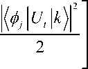
Example. Let the initial state p is shared between subsystems held by A and B, with respective dimensions 2d and d , p = ^jEE(lk^k |0 |t^t |)^ 0 (Ut jk^kU )^ . Here U^ = I and Ux changes the computational basis to a conjugate basis: Vi, k KilU \k\I = -4= . In this example, B is given a random 1d draw k from d states in two possible random bases (depending on t = 0 or 1), while A has complete knowledge on his state.
Let consider for this case the abovementioned expression of Iacc (E). For considered case the ensemble is 113uUJk)f with i =k,t; Pk,t =1 d, ц=I and — Ш = 1.
L 2 d ) k,t 2 d x d
Putting all these in the expression for Iacc (E), we obtain as log2 d+ E aj-1 (ф- lUt lk) |2 log j,k,t 2d
I ( Cl ) ( p ) = max
M
= max M
a log d + E ^
1 ei uk k Г log| ^ . i U - i k >I2
2 j , k , t
Entropies sum where Ea = 1 and V j, t El Ф-М Г = 1 is used to obtain the last line. Since E~ = 1, the second jj k jt jd term is convex combination, and can be upper bounded by maximization over just one term:
I ( Cl ) ( p ) < log d + max1 E| ф| U t l k )Г log | ф| U t l k )|2 .
। ф 2 k , t
Remark. The value -El Ф1 U.k|iog| ф| u»г is the sum of entropies of measuring |ф in the k,t computational basis and the conjugate basis. Such a sum of entropies is least logd . Lower bounds of these types are called entropic uncertainty inequalities (EUI), which quantify how much a vector |ф cannot be simultaneously aligned with states from two conjugated bases. It follows that I(Cl) (p) < — logd . Equality can in fact be attained when B measures in the computational basis, so that I(Cl) (p) = “log d .
The accessible information from m independent draws of an ensemble E of separable states is additive, I acc ( E 0 m m = mIacc ( E ) . It follows I ( Cl ) ( p 0 m m ) = mIacc ( p ) for this case.
Example . If p is a bipartite state on C d 0 C d , then: Tr \pAB — p ® p | < ( 2 d ) 2 ^ 2ln2 • I ( C l ) ( p ) .
It means that when I ( Cl ) ( p ) is small, p must be close to an uncorrelated state (in trace distance).
Thus, when there are no restrictions on the allowed measurement strategy, the classical information about the identity of the state in an ensemble {px, p } , accessible to a measurement is limited by the Holevo bound: Iacc < S(p)-2PxS(px), p = 2PxPx .
For measurements of bipartite ensembles restricted to local operations and classical communications (LOCC) is existed a universal Holevo-like upper bound on the locally accessible information. By “ locally accessible information ” always mean accessible information by LOCC-based measurements. The maximal mutual information I ( X : Y ) accessible via LOCC between A and B satisfies the following inequality:
Z — A, B x where pA and pB are the reductions of pAB — 2 pxpxxB , and px is a reduction of pxB .
x
Example : Interrelations between global and local accessible information . Consider an ensemble of signal states (not necessarily orthogonal or pure) { px , p xB } and pure (not necessarily orthogonal) “detector” states { Pxn } .
Initially, let the signals and the detectors be in a joint state pABCD — 2 pxpxB ® | PxD ффсп | with relative entropy of entanglement EAC : BD ( pABC D) . A measurement restricted to LOCC (between A and B ) and obtaining results j with probability q , will usually leave the detectors in mixed states П cd — 2 px|7• | Фсп >cd |, thus giving the accessible information
С"* u H'S*1 -2q,H({px,}) < H'S*>-2qS,) j W Mj
(equality hold for orthogonal detectors). The general property of relative entropy of entanglement
E aabb ) > E aab ) - E ^ ABB ) , implies that
I ( LOCC ) < H' S* ' +2 qE( , ) - 2 q , S( С ) = H* * + E O - S- .
л ci out Ax \ Ax i \ / Ax \ i zydet i zrdet 77AC: BD / \/
As Sout — 2 qjS (TrD 2 px\j yCcD/ \CcD |)>2 pxE (| ФcD /j = Eout , and Eout < E (pABCD )
LOCC does not increase the relative entropy of entanglement EAC : BD ( pBCD ) ), we obtain:
TT ( Sh ) ,( LOCC )
H - I acc
where A E — E2: - E"C"" ( pabcd ) .
In the case of orthogonal ensembles, H ( S* ) is the global accessible information ( I gl^a ) and for such cases, we have: I gl^a - I LOCC >A E . Thus, in general case the difference between globally and locally accessible information for an ensemble of orthogonal (not necessarily pure) states is not less than the amount of the relative entropy of entanglement, which is created in a global measurement to distinguish the ensemble.
Connections between accessible information and quantum operations
A general quantum process cannot be operated accurately. Furthermore, an unknown state of a closed quantum system cannot be operated arbitrarily by unitary quantum operation. A quantum measurement on the state has been to identify X on the measurement result Y . A good measure of how much information has been gained about X form the measurement is the mutual information H (X : Y) between X and the measurement outcome Y . The mutual information H (X : Y) of X and Y measures how much infor mation X and Y have in common. Holevo’s theorem states that H (X : Y)< X. The quantity X is an upper bound on the accessible information. But the Holevo bound quantity decreases under quantum opera- tions: X
= S ( S ( P ) ) - E P x S ( S ( P x ) )
V x 7
< X = S ( P ) - E P-S ( P * ) I , where s is a quantum operation. V x /
Suppose we will to perform a quantum process, which can be realized by a quantum operation, s . After a quantum process, we find the mutual information decreased, in another word, we find that the information we can gain from the quantum system is less than previous. We know the uncertainty of this quantum states increase because of the decreasing of the accessible information. That is, the result after the quantum operation is unreliable. Also, it tell us this quantum process cannot be operated accurately because if this quantum can be operated accurately, the accessible information would not decrease.
Example : Disentanglement process . Let us consider disentanglement process: s ( P ) ^ Tr. ( P ) ® Tr ( P i2 ) , where д 2 is a pure state of two subsystems. An arbitrary state cannot be disentangled by a physical allowable process into a tensor product of its reduced density matrices. Consider P 2 is a pure state, then the Holevo X -quantity x ( P ) = 0 • After the disentangling process, it has that the
Holevo X -quantity x [ Tr ( P 12 ) ® T ( P ) ] — 0 • [We can prove this by using concavity of the entropy:
S [ E PiPi
V i 7
— E pS ( p ) ]. After the disentangling quantum process, that is
Since the equality holds iff all the states P for which p ; > 0 are identical, we know that a general disentangling quantum states would necessarily increase the Holevo X -quantity. Thus, it tell us a universal disentangling machine cannot exist.
Total, classical and quantum correlations: Examples of interrelations between of covariance, correlation and entanglement measures
It is important in quantum computation to determine how to separate the correlations it contains into a classical and an entangled part.
Remark . In quantum mechanics, most measurement results are represented by the trace of products of observables in certain quantum states. As example, the superposed vectors as Bell states |Ф ±^ ,| ^'/ are maximally entangled in the sense that they are pure on the whole system, and their marginals are maximally mixed:
Tr (Iy1)^1^ ) - Tr (|y‘)(|y*}| ) = Tr (|ф*^|ф±)| ) = Tr (| ф ±^| ф ‘)| ) = 1 1 .
We see readily a string difference between classical states and quantum states. While the marginals of classical pure states are necessarily pure, it is not the case for quantum pure states. This peculiar structure is beautifully described by Schrodinger sense:
”The best possible knowledge of a whole does not necessarily include the best possible knowledge of all its parts .”
Let us demonstrate this approach with simple examples.
Example. Consider a bipartite separable state of the form: pB = У p^ |zAi |® pB , where { i^} are ori thogonal states of subsystem A . Clearly the entanglement of this state is zero. The best measurement that A can make to gain information about B ’s subsystem is a projective measurement onto the states { i^} of subsystem A . Consider the measure of a classical correlation as: CB (pB ) = max 5 (p ) — У pS (p A ) , Bi†Bi i where as above B^Bt is a POVM performed on the subsystem B and p A=
», ( B b P ab BB^ T ab ( B b P ab B B )
is the remain-
ing state of A after obtaining the outcome i on B . Clearly CB ( pB ) = C. ( pB ) for all states pB such that S ( p ) = S ( p ) . The measure is a natural generalization of the classical mutual information, which is the difference in uncertainty about the subsystem B ( A ) before and after a measurement on the correlated subsystem A ( B ) , H ( A : B ) = H ( B ) — H ( BA ) .
Similarly, CB ( pB ) , C, ( pB ) are represented the difference in von Neumann entropy before and after the measurement. These measures CB ( pB ) , C. ( pB ) are non-increasing under local operations. Note the similarity of the definition to the Holevo bound which measures the capacity of quantum states for classical communication. Therefore the classical correlations are given by:
C a ( P ab ) = S ( p b ) —У pS ( p B ) .
z
For this state, the mutual information is also given by: I (p.B ) = S (p ) — У pS (p18 ) . This is to be z expected since there are no entangled correlations and so the total correlations between A and B should be equal to the classical correlations. We now consider the relations between the classical, total and entangled correlations in some simple cases.
Example : Maximally entangled pure state . Let us consider a maximally pure state, | ф ^ ф + |, and the family of states that interpolate between it and its completely decohered state |0A0| + Ц(1|• These are states of the form: pB = p | ф ф ф | + ( 1 — p ) | ф^ ф — |, where — < p < 1 .
The mutual information as a function of p is: I ( p. A = 2 + p log p + ( 1 — p ) log ( 1 — p ) .
The entanglement is: ERi ( pB ) = 1 + p log p + ( 1 — p ) log ( 1 — p ) .
The classical correlations remain constant at: C, ( pB ) = CB ( pB ) = C ( pB ) = 1 .
This is achieved by a projective measurement onto {| GA0|,|1^1 } , and must be the maximum because C cannot exceed one. The total correlations for this case are just the sum of the entangled and the classical correlations, I ( p.B ) = E^ ( P AB ) + C ( P AB ) .
1 — p
Example : Werner state . Consider a Werner state of the form: pB = p| ф фф +-- 1 with
1 < p < 1. 4
3 p + 1
.
The mutual information is: I ( p.B ) = 2 + f log f + ( 1 — f ) log I —-— I , f =
The relative entropy of entanglement is: ERE ( pB ) = 1 + f log / + ( 1 — f ) log ( 1 — f ) .
The classical correlations remain constant at: C, ( pB ) = CB ( pB ) = C ( pB ) .
Any orthogonal projection produces the same value for the classical correlations.
This quantity is called as Cp ( pB ) . Clearly, that: Cp ( pB ) < C ( pB ) .
Example : Symmetric state . The state of the form: pB = p\ 0^|0^0|^0| + (1 — p )| +)|+X+| • Same as above, the state is symmetrical with regard to A and B , so: C, ( pB ) = CB ( p s ) = C ( pB ) .
This state provides a simple example where the states on both sides are non-orthogonal. It is not the measurement, which optimizes the classical correlations.
In these two last examples, Cp ( pB ) + ERE ( pB ) < I ( p.B ) . If the classical correlations are maximized by an orthogonal measurement on one subsystem, the classical and entangle correlations do not account for all the total correlations, and E ( pB ) < C ( pB ) .
Another possible of classical correlations could be based on the relative entropy (see Appendix 1).
Relative entropy as the measure of classical correlations. Just as measures of total and entangled correlations are both relative entropies, I (pB ) = S (pB pA ® p ) and E(p.B ) = min S (pB ||pB ) . ClassiCTAB ED cal correlations could then be given by the relative entropy between the closet separable state, cr*AB, and the product state Qa ® pB, CE = S (^Ab IQ ® pb ).
Example . For a mixture of two Bell states, CRk ( pB ) coincides with CRE ( pB ) = 1 . For the separable state pB = p 1 0^ 1 0^0 1 ^0 1 + ( 1 — p ) | +) | +X+1 , C^ ( pB ) = I ( p.B ) , which makes sense, but there is no entanglement.
Example . For Werner state, the relative entropy of classical correlations remains constant at Cre ( Pb ) = 0.2075 . Therefore for low values of p , CRДpB ) > EKДpB ) , whereas for high values, CR e ( Pb ) < Ere ( pB ) , so that the two types of correlations do not sum to the total.
In general, we have the inequality as I ( p.B ) > EKE ( pAB ) + C^. ( pB ) , so that the two types of correlations do not sum to the total.
Remark . Thus, the measure of the classical correlations of a bipartite state pB is a distance between the nearest state p * of pB and p *^ ® p B , that is relative entropy C ( pB ) = S ( p * 1 1 p A ® p* B ) .
This measure of classical correlations, and similar measures based on the distance between p* and Pa ® Pb such as C2 ( Pab ) = S (P‘| Qa ® Pb ) are equal to the von Neumann mutual information, I ( Pb ) = S (p ) + S (p ) — S (pB ) = S (pBpA ® p ) for a set of separable states. A measure of the classical correlations based on the maximum information that could be extracted on a subsystem B of pAB s ( Pb )—E PS ( Pb )
by making a measurement on the other subsystem A described above so: x = max B AiAi† is not proved to be symmetric under interchange of the subsystems A and B and even if it could increase under LOCC this should be expected for classical correlations.
Another measure of classical correlations in quantum state can be defined as the difference between total correlations measured by the von Neumann mutual information and the quantum correlations measured by the relative entropy of entanglement: V ( pB ) = S ( pB ||p ® p ) - min S (pB ||p*) , where D is the set of all separable states in the Hilbert space, on which pB is defined. This measure of the classical correlation is superadditive in the sense that V (p ® p) > 2 V (p) due to the fact that the mutual information is additive, whereas the relative entropy of entanglement is subadditive.
For pure states, all the measures of the classical correlations including this measure are equal to the von Neumann entropy of the subsystems A or B : S ( p ) = S ( p ) . According to the definition of the classical correlation, all the correlations contained in separable states are classical.
Covariance and entanglement . In quantum mechanics it is long recognized that there exist correlations between observables, which are much stronger than classical ones. These correlations are usually entanglement, and cannot be accounted for by classical theory.
-
A . Covariance . The notion of classical covariance of two random variables can be naturally extended to quantum mechanics, when the probability is replaced by a quantum state (density matrix), and the random variables by observables. Thus let H be the Hilbert space of a quantum system, let L ( H ) be the real linear space of all observables on H . Let p be a quantum state (mixed state, in general), then for any two observables A and B , their covariance Cov p ( A, B ) is defined as:
In particular, the variance of A in the state p is defined as:
VarpA = Covp ( A, A ) = Tr ( p A 2 ) - ( Tr p A ) 2 .
Example . When p is diagonalized, in spectral decomposition form, p = ^ X | Uj ^ U^ | and p is nondegenerate and thus { Uj ^} constitutes an orthonormal base, we have
Covp ( A,B ) = Z X uj | AI uk Wk B |u j) -Z Xj^k uj AuWWWW j, k j, k and
VarpA = T , X K u| A I и > |2 - Z Wk u j \AW W A\W j , k j , k
= Z j —(ul A lu)- E jiMWiWk AM
-
j , k 2 j , k
Let [A,B] = AB — BA denote the commutator. Since Covp (A,B) — Covp (B, A) = Tr (p[A,B]), and Covp (•, •) maybe viewed as an inner product, by Schwarz inequality, we have
Var p A • Var p B >1 | Tr ( p [ A , B ])| .
This is the conventional Heisenberg uncertainty relation.
-
B . Interrelations between covariance and entanglement . Physically, covariance is usually used to characterize correlations between two observables in a given quantum state. Alternatively, it can be used to characterize the intrinsic correlations of a quantum state, given the two observables fixed. The situation is usually as follows. Let there be given two quantum systems H and H and two observables a and b for the two quantum systems respectively. Then A = a ® I 2, B = I ® b are two observables for the composite quantum system H , ® H2, and they commute. Now let p be any quantum state of the composite quantum system, then Cov p ( A, B ) maybe used as a measure to quantify the “correlation strength” of the state p . The observables A and B serve here as testing observables.
Example . Let | ^ ) e H , and | ^ 2) e H 2 be two quantum states, and let the composite quantum state
I ^ ) = I ^ i) ® I ^ 2) e H ]® H 2 be a product state. For p = | ^) ^ |, then we have Cov ( A,B ) = 0 . Let now H j= C 2 , H 2= C2 , and the composite quantum system be H j® H 2= C2 ® C2 . Let
A = c r z ® I 2, B = I ® ^ . Then sup Cov w .( A,B ) = 1, inf Cov.x, . ( A,B ) =- 1 . The maximum
^ w value is achieved iff: |^) = —^=(ea |00) + ев |11)) and the minimum is achieved iff:
| ^ = -^=( C" |01) + ee |10)) . Here a and в are any real constants. Thus maximally entangled states as
Bell states maximize the magnitude of the covariance Cov ( A . B ) •
The distinctions between classical and quantum correlations are fundamental and subtle, and it is a difficult and thorny problem as how to distinguish them. In this respect, the conventional covariance often gives ambiguous results. Let demonstrate this point by an example.
Example . Let as above H t= C 2 , H 2= C2 , and the composite quantum system be
H j® H 2= C2 ® C2 = C 4 . Take a quantum state p = 2 (100^^00] + 111^11 1) and
A = ( T z ® I 2, B = I ® ^ . Then in the canonical base { 00),|01),|10),|1) } , we have
Г 1
p ’=2
0 01
0 00
0 00
0 01
We readily compute Covp• ( A, B ) = 1 •
The state p is a mixture of two disentangled (product) states, while p' is a Bell state, which is maximally entangled, and the covariance cannot distinguish them. In this sense the conventional covariance has a limited use in characterizing entanglement.
We will investigate entanglement by means of another “covariance” measure, the Wigner-Yanase-Dyson correlation, which is of an informational origin connected with Fisher information and skew information. This correlation measure has some advantages over the conventional covariance in quantifying entanglement (see Appendix 1).
Wigner-Yanase-Dyson (WYD) skew information measure
In the study of measurement theory from an information-theoretic point of view, Wigner and Yanase introduced the quantity:
which they called skew information (the bracket [ • , • ] denotes commutator), as the amount of information on the values of observables not commuting with K (which may be a Hamiltonian, a moment, or other conserved quantity). Alternatively, I ( p , K ) may be interpreted as a measure of non-commutativity between p and K with asymmetric emphasis on the state p and on the conserved observable K .
Properties of the skew information are as following: (i) constant for isolated systems; (ii) decreases when two different ensembles are united that means the information content of the resulting ensemble should be smaller than the average information component of the component ensemble; and (iii) is additive, namely, the information content of two independent pairs is the sum of information of the parts.
The skew information is later on generalized by Dyson to
The WYD conjecture concerning the convexity of Ia ( p , K ) .
The Wigner-Yanase skew information can be rewritten as following:
In particular case, if p = | ^ ^ | is a pure state, then
Here Ap K is the variance of the observable K in the state p .
Therefore, for pure states, the Wigner-Yanase skew information reduces to variance. When p is a mixed state, we have: Ap K > I ( p , K ) .
-
A . Interrelations between quantum Fisher’s information and quantum Wigner-Yanase skew information . In fact, the notion of skew information is very similar to the well-known notion of Fisher information originated from statistical inference. Among concepts describing contents of quantum mechanical density operators, both the Wigner-Yanase skew information and the quantum Fisher information defined via symmetric logarithmic derivatives are natural generalizations of the classical Fisher information.
We will establish a relationship between these fundamental quantities.
Recall that the Fisher information of a parameterized family of probability densities { pg : 9 e R } on
R is defined as
I f ( P . ) = 4 J r ^ dx = 1 J R ^ log p M p . ( x ) dx
j 4 0 J is intimately related to the Shannon entropy.
Remark . When we pass from classical theory to quantum mechanics, the integral is replaced by trace, and the probability densities are replaced by density operators.
The Fisher information for a family of quantum states p is defined as
which may be viewed as a generalization of the classical Fisher information to quantum case.
In particular, if p satisfies the Landau-von Neumann equation:
where 9 e R is a (temporal or spatial) parameter, and K may be interpreted as the generator of the temporal shift or the spatial displacement, then p = e - i 9 Kpe9 K , and
-—-=ie ,/p-KJe which in turn implies that If (p ) = 81 (p, K) .
Therefore, the skew information is essentially a particular kind of quantum Fisher information. In general case, the quantum Fisher information and the Wigner-Yanase information are related by inequalities:
Example : Two-level quantum system . The quantum state Hilbert space is C 2 . A general density opera-
5 i7 1 ( 1 + r tor p on C 2 for some r = (r, r, r) e R3, | r| = rr12 + r2 + r2 < 1 is of the form: p = —
2 ( r l + ir
r l - ir 2 1 - r
.
1 - I r l 1 + I r l
The eigenvalues of p are ^ =—-— and ^ = —-—. Let the corresponding eigenvectors be ^ and^, thenp = ^ |^)(^ | + ^ |^)(^ |. Consequently, and
Thus IF ( p, K ) may vary continuously from Iw ( p, K ) to 2 Iw ( p, K ) . Moreover, in this case, if ^ |K | ^ 2) ^ 0 and K does not commute with p , then IF ( p ,K ) = Iw ( p ,K ) iff | r | = 1 , that is, p is a pure state.
-
B . The Wigner-Yanase correlation . Motivated by Fisher information a skew information, the Wigner-Yanase correlation can be introduced as following (in analogue with the measure of correlation A^ K ):
Cor p ( A, B ) = Tr ( pAB ) - Tr ( ^A^B ) .
In particular,
I ( p,K ) = Corr p ( A, A ) = Tr ( pA' ) - Tr ( .JpA ) = - 1 Tr [ ^p, A ]
is exactly the skew information introduced by Wigner and Yanase.
Since Corrp ( A,B ) — Corrp ( B , A ) = Tr [ A,B ] and Corrp ( ■ , • ) maybe viewed as an inner product, by the Schwarz inequality, we also have:
I ( p .A ) • I ( p ,В ) >- Tr [ A , В ] .
This inequality is more strong than the Heisenberg uncertainty relation since: Var A > I ( p , A ) . Thus, just like the Fisher information, the Wigner-Yanase correlation can also to improve the conventional Heisenberg uncertainty relations (see Appendix 2).
-
C . The Wigner-Yanase correlation and covariance . The conventional covariance and the Wigner-Yanase correlation are two different correlation measures: Wigner-Yanase correlation has more information character and there are some intrinsic relations between them.
The inequality Covp ( A, A ) > Corrp ( A, A ) is true, but Cov ^ ( A, A )| > Corr ^ ( A, A )| and it is not true in general: the magnitude of the conventional covariance can be less, or large, than the Wigner-Yanase correlation.
Example. Let v 0 ^ J’ [ a a22,
Г b
I b
b 22 J
Here 2 + 2 = 1, A > 0, 2 > 0 and avpa22,bpb22 are all real numbers, while a and b may be com- plex. Then
In particular, if a and b are real, then Cov ^ ( A , A )| > | Corr p ( A , A )| iff
However, if p is a pure state, these two correlation measures coincide: Covp ( A, B ) = Corrp ( A , B ) for any observables A and B .
-
D . The Wigner-Yanase correlation and entanglement. Let p , p and A , B be the same as above:
4 1 0 0 0 ) ( 10 0
1 )
1 0 0 0 0 ,1 0 0 0
p = - , p = -
2 0 0 0 0 2 0 0 0
0
0
, 0 0 0 1 J ( 10 0
1 J
Then we may readily compute Corrp ( A, B ) = 0, Corrp , ( A, B ) = 1 . Thus the Wigner-Yanase correlation indeed distinguishes between the mixture of disentangled states (classical correlation) and the maximally entangled Bell states (quantum correlation).
Example : H = C 2 , H2 = C 2 and the composite quantum system H ® H2 = C 2 ® C 2 = C 4 . Take a quantum state
Let us as above A = crz ® I 2, B = I ®CTZ . Then in the canonical base { 00^,10^,110^,110 } , we have
( 3 0 00
4 0 0 00
^0 0 01
Tr ( p A ) = Tr ( p B ) = -, Tr ( p AB ) = 1 Cov p ( A , B ) = - = 0.75
The calculation leads to 2 , thus
|
f 1 |
0 |
0 |
1 |
|
|
74 - 272 |
74 + 272 |
|||
|
1 |
1 |
|||
|
IT |
0 |
2 |
2 |
0 |
|
U = |
A |
1 |
1 |
A |
|
0 |
2 |
2 |
0 |
|
|
72 - 1 |
0 |
0 |
72+ 1 |
|
|
4 74 - 272 |
74 + 272 |
This is in sharp contrast with the covariance: Cov ( A , B ) = 0.75 . Indeed, the state p is half mixture of a disentangled state 1 00^ ^00 1 and an entangled state: I ф + \ /ф + I.
Thus the entanglement in p should be less than 0.5 if we take Ф ) (a bell state) as a state with a unit of entanglement (indeed, Cov |ф+ ^ф+|( A , B ) = Corr ф ^ф+|( A , B ) = 1 ) and assume reasonable that classical mixing will reduce entanglement (mixing the disentangled state 00 00 with the entangled state I ф + дф' I will corrupt the entanglement).
Efficient measurements and bounds on the accessible mutual information
In general case, when a measurement is made on a quantum system in which classical information is encoded, the measurement reduced the observer’s average Shannon entropy for the encoding ensemble. This reduction, being the mutual information, is always non-negative. For efficient measurements the state is also purified; that is, on average, the observer’s von Neumann entropy for the case of the system is also reduced by a non-negative amount.
By rewritten a bound derived by Hall, which is dual to the Holevo bound, one finds that for efficient measurements, the mutual information is bounded by the reduction in the von Neumann entropy.
-
A . Hall ’s dual Holevo bound is as following:
Thus,
p =
f 72 + 1 ) 2
1 2T2 ,
У2 - 1 )
( 72 + 1 ) 2 (72 - 1 ) 2
( 272 ) 2 ( 272 ) 2
(7 2 + 1 )2 ( - 1 ) 2
( 272 ) 2 ( 272 ) 2
(72 + 1 ) 2 (72 - 1 ) 2
( 272 ) 2 + ( 272 ) 2
Simple calculation leads to: Corrp ( A , B ) = —
—
0.15 .
A I . = H ( I : J ) < S ( p^ Q j S j
' JpUj^
Q , = Tr L U , p ] ; и , = A ,
where Q is the probability that outcome j will result; each of operators A corresponds to the measurement outcome, and the outcomes are therefore labeled by j .
-
B . Schumacher-Westmoreland-Wootters (SWW) bound . The Holevo bound and Hall’s bound, may both be derived from the more general SWW-bound
a i . < s ( p ) -Z pS ( p , ) -^ Q , s ( p ') — Z j , ( p , )
i , L i
X — quantity where all quantities are as defined above, and the quantity p‘ is introduced, which is the final state that the receiver would have had, if he knew that the initial state was p .
Thus, p i, =
A j pjA ■ Q ( A )
, where Q ( ,|, ) is naturally the probability density for the measurement outcomes,
given that the initial state is p . Because of the final term on the right-hand side of this inequality, this bound is, in general, stronger than the Holevo bound.
Remark . The expression in the square brackets
S ( p O-Z p4s ( p i )
is the Holevo X quantity for
the ensemble 8., which results from measurement outcome , . Thus their bound may be written as: A Iin < X[8] — ZQjX [8 ] . Now, X [8 ] is the Holevo bound on the information that the receiver could j extract when making a subsequent measurement after obtaining result j .
While A I in quantities the information which the observer obtains about the initial preparation, there exists another quantity which can be said to characterize the average amount of information which receiver obtains about the final state which he is left with after the measurement. Denote this by AIn , expression for which is as:
j
This is the average difference between the receiver’s initial von Neumann entropy of the quantum system, and his final von Neumann entropy. A more fundamental difference between A I in and A I. is that the former is the average change in the observer Shannon entropy regarding the ensemble, where as the latter is the average change in the observers von Neumann entropy regarding the overall state of the quantum system.
That is, for any ensemble 8 , AIin = ^ A H ( 8 )^ and A I^n = ^ A S ( 8 )^ , and the result is AIin < A I^n .
One can interpret this as saying that the observer cannot learn more about the classical information encoded in a quantum system than he learns about the state of the quantum system. This provides a physical interpretation for Hall’s bound.
Further, this bound can only be saturated when all operators U. = A j A. commute.
Remark . One consequence of the relation A Iin < A I^n is that, if we choose an ensemble, which has the maximal accessible information for a fixed p , we can only obtain all this information if all the final states are pure. Measurements, which leave the final state impure, leave some information in the system. That is, if 16
the final state is mixed, in general it depends on the initial ensemble, and as the result subsequent measurements can obtain further information about the initial preparation, whereas this is not possible if the final state is pure.
For a given p not all ensembles have an accessible information equal to S ( p ) . In fact, this is possible if the encoding satisfies special conditions; in general, incomplete measurements will not even extract the accessible information from an ensemble. Consider the final states, p ‘ , which result from the measurement. Each of these consists of an ensemble, г ; over the states p^ , and p ' = E p ( i\ j ) p^ j • i
Since these ensembles consist of states indexed by i , they can, in general, be measured to obtain further information about the initial preparation.
Since the accessible information is the maximal amount of information that can be obtained about i by making measurements, we have the inequality:
A I„ ( г, U ) Iю ( г ) - E Q , M., ( г , ) .
Thus, the amount of extracted information by measurement U , A Iin ( г , U ) , can only be equal to A Iacc ( г ) if the amount A IQcc (p ) are zero for all j . If p ‘ is pure, then A IQcc (p ) is zero. If p ‘ is not pure, then the accessible information of г is only zero if, for any given j , the p^. are the same for all i .
The SWW bound shows that, if the initial ensemble г is chosen so that its accessible information is maximal [i.e., equal to х [ г ] ], then the information obtained by an incomplete measurement will be reduced by the maximal amount of information which could be accessible from the final ensemble г , and not merely the actual information available in these ensembles, which would imply the bound given in:
In general, there is a gap between the information lacking in an incomplete measurement, and that which can be recovered by subsequent measurements: no matter what incomplete measurement is performed on it, the information which is not retrieved by the measurement can always be extracted by subsequent measurements.
Remark . For inefficient quantum measurements, however, the inequality A Iin < A I^n does not hold. The reason for this is that for inefficient measurements A I/7jj can be negative (whereas A Iin is always nonnegative). An example of such a situation is one in which the initial state p is not maximally mixed, and the observer performs a von Neumann measurement in a basis unbiased with respect to eigenbasis of p . If the observer has no knowledge of the outcome, then his final state is maximally mixed. Further, if one mixes this measurement with one whose measurement operators commute with p , it is not hard to obtain a measurement in which both A Iin and A I/7jj are positive, but which violates the inequality A Iin < A In .
These quantities are useful when considering quantum state preparation and, more general quantum feedback control.
Information (communication) capacity of quantum computing
Any computation (both classical and quantum) is formally identical to a communication in time. By considering quantum computation as a communication process, we relate its efficiency to its classical communication capacity. At time t = 0, the programmer sets the computer to accomplish any one of several possible tasks. Each of these tasks can be regarded as embodying a different message. Another programmer can obtain this message by looking at the output of the computer when the computation is finished at time t = T. Computation based on quantum principles allows for more efficient algorithms for solving certain problems than algorithms based on pure classical principles. The classical capacity of a quantum communication channel is connected with the efficiency of quantum computing using entropic arguments.
This formalism allows us to derive lower bounds on the computational complexity of quantum control and search algorithms in the most general context.
Communication model of quantum computing
In this model two programmers (the sender and the receiver) and two registers (the memory (M) register and the computational (C) register) are applied. The sender prepares the memory register in a certain quantum state i , which encodes the problem to be solved. For example, in the case of search, this register will store the state of the list to be searched. The number N of possible states i will be limited by the target list that the given computer could search. The receiver then prepares the computational register in some initial state p0 . Both the sender and the receiver feed the registers (prepare by them) to the quantum computer. The quantum computer implements the following general transformation on the registers:
(I # I) „ ® pC ^(1 -X- I).„ ® Up W - where pc (i) = Utp0Ut^ is the resulting state of the computational register that contains the answer to the computational basis and is measured by the receiver according to measurement basis (as exam- ple- (I °M0 ) or
(l °') =^ (10+l I) >10^ (I °)-11)?
). The quantum computation should also work for
N any mixture E Pi (l # Dm -where p- are probabilities. For the sender to use the above computation as a i=1 “ communication protocol, he has to prepare any one of the state with an a priori probability p . The
N entire input ensemble is thus: E Pi (| -) (-1) ® P 0 . Because of the quantum computation, this becomes i=1 " "
NN i =1 - - =1 -
Whereas before the quantum computation, the two registers were completely uncorrelated (the amount of mutual information is zero), at the end, the amount of the mutual information becomes: I MC : = S ( p M ) + S ( p c ) — S ( p MC ) = S ( p c ) - E PS ( p c ( i ) ) - where p . and p c are the reduced density operators for the two registers, pc is the density operator of the entire ( M + c ) — system, and S ( p ) = — Tr ( p log p ) is the von Neumann entropy.
Remark . The sender conveys the maximum information when all the message states have equal a priori probability (which also maximizes the channel capacity). In that case the mutual information (channel capacity) at the end of the computation is log N .
Thus, the communication capacity I , defined above, gives an index of efficiency of a quantum computation : A necessary target of a quantum computation is to achieve the maximum possible communication capacity consistent with given initial states of the quantum computing .
Remark . If one breaks down the general unitary transformation U of a quantum algorithm into a number of successive unitary blocks, then the maximum capacity may be achieved only after the number of applications of the blocks. In each of the smaller unitary blocks the mutual information between M and C registers (i.e., the communication capacity) increases by a certain amount. When its total value reaches the maximum possible value consistent with a given initial state of the quantum computing, the computation is regarded as being complete.
Application of information formalism to any general quantum search algorithm
Any general quantum algorithm has to have a certain number of queries into the memory register. This is necessitated by the fact that the transformation on the computational register has to depend on the problem at hand, encoded in the state i . These queries are considered to be implemented by a block box into which the states of both the memory and the computational registers are fed. The number of such queries (needed in a certain quantum algorithm) gives the black box complexity of that algorithm and is a lower bound on the complexity of the whole algorithm.
N
If the memory register was prepared initially in the superposition ^| 0, then, in a search algorithm, i =1 ~
O ( -JN ) queries would needed to completely entangle it with the computational register ( Ambainis , 2000).
This gives a lower bound on the number of queries in a search algorithm. We can calculate the change in mutual information between the memory and the computational registers in one query step. The number of queries needed to increase the mutual information to log N (the perfect communication between the sender and the receiver), is then a lower bound on the complexity of the algorithm.
^14^' z.. —
Any other unitary transformation performing a query matching the states of the M and the C registers could be constructed from the above type of queries.
We can to put a bound on the change of the mutual information in one such black box step. Let the memory states i be available to the sender with equal a priori probability so that the communication
1N capacity is a maximum. The initial ensemble of the sender then is — ^(| i)(i |)M • Let the receiver prepare the register C in an initial pure state | i/0 ). In fact, the power of quantum computing stems from the ability
1N of the receiver to prepare pure superposition of form ,— ^ | у ^c . This is an equal weight superposition of
V N j = 1
all C .
This can be done by performing a Hadamard transformation to each qubit of the C register. In general, there will be many black box steps on the initial ensemble before a perfect correlation is set up between the M and the C registers. Let, after the k — th black box step, the state of the system be:
N
N i =1 - j
The ( k + 1 ) — th black box step changes this state to
N
N i =1 - j
Thus, only the difference of mutual information between the M and the C registers for states are evaluated.
Remark . This difference of mutual information can be defined as follows. The amount of information lost may be quantified by the difference in mutual information between the respective states. Mutual information is a measure of correlation between the memory M and the C registers, giving the amount of information about the C register, which may be obtained from a measurement on the M register. The quantum mutual information between the M and the C registers is defined as above. The mutual information loss for the step k is A Ik = S ( p k ) . Then the difference of mutual information between the step k and the step k + 1 can be shown to be the difference: | A Ik+ , — A Ik | = S ( p k + 1 ) — S ( p k )|.
Remark . To understand how the entanglement (quantum correlation) between the M and the C registers varies as we vary the density matrix for the combined system, we need to introduce some distance measures on density matrices. We will make use of three closely related distance measures: the trace distance Tr ( p , k ) , the fidelity F ( p , a ) , and the Bures distance D ( p , а ) . These distances between density matrices p and a are defined to be as follows:
The trace distance Tr ( p , а ) is a metric on the space of density matrices and it is nonincreasing under quantum operations: T ( L ( p ) , L ( a ) ) < T ( p , T ) for all density matrices. The Bures distance D ( p , а ) is also to be a metric on the space of density matrices and agrees with the trace distance for pure states. Bures metric does not increase under general complete positive maps (which is what the query represents when we trace out the M register). For our purpose, it is especially important to note that this is true for the case where L is a partial trace operation, as the partial trace is a trace – preserving quantum operation. The fidelity F ( P , a ) is not a metric and for pure states | ^ and | ф reduces to the overlap between the states,
F ( ^ , Ф ) =\ Mk I-
It was proved a useful continuity relation relating trace distance and entropy.
Fannes’ inequality states that for any density matrices p and a such that where d is the dimensional of the Hilbert space, and h ( x) = — x log x.
Recall that T ( p, a ) < D ( p , a ) the quantity |A Ik+ j—A Ik | = S ( pck + 1 ) — S ( pck )| is bounded from
Fannes’ inequality by
I S ( p C + 1 ) — S ( p C )|< D 2 ( p C , p C + 1 ) log N — D 2 ( p C , p C + 1 ) log D 2 ( p C , p C + 1 ) .
It can be shown that F2 ( p0, p1 ) > ——— from which it follows that the change in the first step:
The change S ( p k + 1 ) — S ( p k )|
in the subsequent steps has to be less than or equal to the change in the first step. This is because Bures metric does not increase under general complete positive maps as above is mentioned. Any other operation performed only on the C register in between two queries can only reduce the mutual information between the M and the C registers. This means that at least O (VN) steps are needed to produce full correlations (maximum mutual information of value log N as a measure of a maximum entanglement) between two registers. This gives the black box lower bound on the complexity of any quantum algorithms.
Intelligent coherent states with minimum uncertainty and maximal information
The minimum-uncertainty coherent states (as example, for the harmonic-oscillator potential) can be defined as those states that minimize the uncertainty relation of Heisenberg (leading to the equality in the uncertainty relations), subject to the added constraint that the ground state is a member of the set. They are considered to be as close as possible to the classical states. Beyond the harmonic-oscillator system, coherent states have also been developed for quantum (Schrodinger) systems with general potentials and for general Lie symmetries. These states are called (general) minimum-uncertainty coherent states and (general) displacement-operator coherent states. There is also a different generalization of the coherent states of the harmonic-oscillator system. This is the concept of “squeezed” states. (Squeezing is a reduction of quadrature fluctuations below the level associated with the vacuum.)
-
A . The even and odd coherent states for one-mode harmonic oscillator were introduced in 1970s. These states, which have been called Schrodinger cat states, were studied in detail. These states are representatives of non-classical states. Schrodinger cat states have properties similar to those of the squeezed states, i.e. the squeezed vacuum state and the even coherent state contain Fock states with an even number of photons.
Definition : Intelligent states are quantum states, which satisfy the equality in the uncertainty relation for non-commuting observables.
In quantum mechanics two non-commuting observables cannot be simultaneously measured with arbitrary precision. This fact, often called the Heisenberg uncertainty principle, is a fundamental restriction that is related neither to imperfection of the existing real-life measuring devices nor to the experimental errors of observation. It is rather the intrinsic property of the quantum states itself.
The uncertainty principle provides (paradoxically enough) the only way to avoid many interpretation problems. The uncertainty principle specified for given pairs of observables finds its mathematical manifestation as the uncertainty relations. The first rigorous derivation of the uncertainty relation from the basic non- commuting observables (i.e., for the position and moment, [5c, p] = ih) is due to Kennard (1927). This derivation (repeated in most textbooks on quantum mechanics ever since) leads to the inequality: A5cAjp > ^ Й . In fact, it can be considered as a simple consequence of the properties of the Fourier transform that connects the wave functions of the system in the position and momentum representation (more general form of uncertainty inequality with Wigner-Yanase-Dyson skew information in Appendix 2 are described).
-
B . It is possible to present quantum uncertainty relations (UR) in terms of entropy or information (“en-tropic UR” –EUR). The usual “standard UR” (for standard deviations)
( A , A )2( A , B ) 2 >4| ([ A,B ] -) ,
+
1 (( A, B } )
4 >+/ ф
—2< A \ B),
(note that the second term in this inequality represents the covariance, or correlation, cov, (A,B) :=1 ф|AB + BA|ф — ф|A |фф|B |ф)
between the observables A and B in the state | ^ ) presented by an inequality of the entropic form
s(A)+ S(B )> SAB or in information form as more adequate expressions for the “uncertainty principle”.
It is known that given two non-commuting observables, we can derive an uncertainty relation for them and the class of states that satisfy the equality sign in the inequality are called intelligent states (see, Definition).
Example . If we have any continuous parameter X
generator of the
parametric
evolution, then
and any hermitian observable A ( X ) which is the UR give us ^A A ( X )^ A X > —, where
X
j AA ( x ) dx
X 1
is the parameter
average of the observable uncertainty and
A X = — ( x — X ) is the scaled displacement in the space of the conjugate variable of A . This generalized s 0
UR would hold for position-momentum, phase-number or any combinations. For the case when initial and final states are orthogonal we know that all states of the form
Iv (X))=11
e
aj
^
are the only intelligent states which satisfy the equality ^A A ( X ) AX = — .
However, these states do not satisfy the equality when the initial and final states are non-orthogonal. In this case, if the generator of the parametric evolution A can be split into two parts A0 + A1 such that Ao has a complex basis of normalised eigenvectors {^ )} which degenerate spectrum {a0}, with 1 a set of quantum numbers and Ax has matrix elements (Ax )u = 0 = (A1 ) ^ , and (Ax )„ = (Ax ).. = ax, then all states of the form
cos a
| V - i sin I '
are intelligent states for non-orthogonal initial and final states.
-
C. It has been shown that the “Everett (entropic) UR” implies the famous Heisenberg UR as
^
AqAp > —. We shall compare various characterisations of maximal information and point out their con nection with “minimum uncertainty”. In the following we restrict ourselves mainly to “simple” observables (defined on the smallest non-trivial Boolean algebra Z = {0, a, — a,1}): we are interested in information with respect to single effect
Non-commutativity or incompatibility of (unsharp) properties E and F will, in general, exclude the possibility of measuring or preparing both of them simultaneously. In particular, if E = E Q ( X ), F = FP ( Y ) are position and momentum spectral projections associated with bounded measurable sets X , Y , then E Q ( X ) л Ep ( Y ) = 0 holds or, equivalently
Thus “certain” position and momentum determinations exclude each other, and the question arises as to what “degree of uncertainty” they can be “known” simultaneously. One may take any reasonable characterisation of maximal joint knowledge, or joint information. In this case above mentioned statement can be put into the following equivalent form
11 | E ф + F ф < 2
1ч e • F < 1
The “state of maximal information” can be defined through three values.
The first expression E + F can be maximised and an explicit construction procedure for the corresponding “state of maximal information” has been given below. Here we shall study the question of maxima for this quantity as well as for E ^ • F^ and for I ( E ) + I ( F ) for an arbitrary pair of effects, E and F . In particular, we shall show that each quantity can be maximal only if there exist states which lead to minimal uncertainty product in UR.
Furthermore, in the case of projections the maxima of I ^ ( E ) + 1^ ( F ) (if they exist) coincide with those of one of the quantities E ^ + F and E ^ • F ( e v e { E , E ' } , F n e { F , F ' } ) .
For maximal E^ + F the variation of ^|E| ^ + ^ F \^ — —^|^ must vanish which implies the following equations: ( E + F ) ^ = ( E ^ + F ) ^ . Multiplying with E or with F and taking the expectations yields
Электронный журнал «Системный анализ в науке и образовании» which leads to a minimal UR: (a^ E ) 2 • (a^ F ) 2 = [ cov^ ( E , F ) ] 2 .
Similarly, maximising the product E ■ F(p gives (F^E + E^F) ^ = 2Еф • Fv | ^ and which leads again to a minimal UR, Еф ^ 0 ^ F .
Finally, maximal information sum I ( E ) + I ( F ) will be realised in states satisfying
Generally this equation contains all stationary points, e.g. the minimum Еф = E’ф = Fp = F' ф = — , or the joint eigenstates. Since we are looking for states of maximal information with respect to positive outcomes for E , F we shall assume Еф > — and FT > — . Then this equality implies:
ln
E Ф )
F )
Ф
F'
F ф 7
ln and а(АфE)2 = —(a^F)2 = - cov(E, F) which again gives rise to the minimal uncertainty product in UR.
We have thus shown that all three notions of maximal information are consistent in so far as they imply minimal uncertainty product.
Example . Let E , F denote position and momentum spectral projections, respectively: E = E® ( X ), F = FP ( У ) . The sum of probabilities Еф + F p has been shown to be maximal in the state
Ф = ^ mm with k min> =
1/2
1 + ati la 2
V au о 7
1 - a о
V 2 ( 1 - a 02 ) 7
1/2
provided that X , Y are bounded measurable sets. Here a 2 is the maximal eigenvalue of the compact operator (FEF) and g is the corresponding eigenvector satisfying
FEF\g о) = a 02 1 g o\F|g о) = | g o) ,||| g оЯ2 = 1 .
It is clear from above description that (Pmn must be an eigenstate of ( E + F ) . This can also be seen directly in the following way. Introduce
I f о) = a 0 -1 Eg о) , II f .IL2 = a« кg о I FEF|g о) = 1, E|f о) = | f 0 .
Then we have
EFE\fф = a о2 f ,) ,| g 0) = a-' F\f^
and ^n can be written in the symmetric form min
72 ( 1 + a 0 )
We conclude that (Pmn maximises all the three quantities (E • F ) , ( Еф + Еф ) and ( I ( E ) + 1 ( F ) ) , and it minimises the uncertainty product ЕфE • ЕфF .
Thus maximal information (minimal entropy) and minimal uncertainty can be achieved on intelligent coherent states and will again coincide.
Conclusions
We discuss the role of entropy changing in quantum evolution as information data flow processing and how the classical and quantum information amount changes in the dynamics of some quantum control algorithms. We introduce the following qualitative axiomatic description of dynamic evolution of information flow in QA’s:
-
(1) The information amount of successful result increases while the quantum algorithm is in execution;
-
(2) The quantity of information becomes the fitness function for recognition of successful results and introduces a measure of accuracy for them: in this case the Principle of Minimum of Classical / Quantum Entropy corresponds to recognition of success results on intelligent output states of quantum algorithm computation;
-
(3) If the classical entropy of the output vector is small, the degree of order for this output state is great and the output of measurement process on intelligent states of quantum algorithm’s gives us the necessary information to solve with success the initial problem.
These information axioms mean that the quantum algorithms should automatically guarantee convergence of information amount to a precise value. This is a necessary condition in order to get robust and stable results for fault-tolerant computation in quantum control.
-
Appendix 1: Relative entropies and divergence functions
Divergence functions can be used to define metric tensors on the space of invertible states of a quantum system. These divergence functions play a central role in quantum information theory.
As an example, let consider the quantum relative entropy, also known as von Neumann relative entropy:
-
S vN ( P C ) = ТГ Р ( log P - lOgс ) (A1.1)
It is the quantum generalization of the Kullback-Leibler divergence function used in classical information geometry and, in the asympotic, memoryless setting, it yields fundamental limits on the performance of information-processing tasks. Another important family of relative entropies is the q-Renyi relative entropies ( q -RRE)
(A1.3)
and the potential function of the Wigner-Yanase metric tensor:
S wy ( p |c ) = 4 [ 1 - Tr ( p c * ) ] (A1.4)
Several efforts were done in order to find a common mathematical framework to unify this plethora of different divergence functions. A first (partial) result was achieved by the q-quantum Renyi divergence ( q -QRD)
S QRD ( p с ) = “[log Tr
1-q 1-q c 2 q pc 2 q
(A1.5)
where again q e ( 0,1 ) о ( 1, го ) . However, it has two important limitations: the data processing inequality (DPI)
(A1.6)
where Ф is a completely positive trace preserving map (CPTP) acting on a pair of semidefinite Hermitian operators p and c , is not satisfied for q e ( 0/Л ) and it does not contain the q -RRE family.
Recently, a new family of two-point functions which includes all the previous examples was defined. It is the so-called q-z-Renyi Relative Entropy ( q-z- RRE)
S qz ( p к ) = ’log Tr [ c 2 z p z c 2 qz ) (A1.7)
q -1 V that can be recast as:
1 ^ q 1 - q A z
Sq, z ( p ^ ) = --- 7lOS ТГ c z p z (A1.8)
q -1 V)
Remark: In general, the product of two Hermitian matrices is not a Hermitian matrix. However, the q product matrix cz p z has real, non-negative eigenvalues, even though it is not in general a hermitian matrix. It means that the trace functional
/ q fq, z ( p Ь ) = ТГ c z p z
(A1.9)
is well defined as the sum of the the z -th power of the eigenvalues of the product matrix and it can be developed in Taylor series.
In particular limits of the parameters q and z it is possible to recover the q- RRE family
S q ,1 ( p к ) : = lim S q , z ( p к ) = S RRE ( p k ) = log Tr ( p q c 1 - q ) (A1.10)
z ^ 1 q - 1
the q- QRD family
Sq , q ( P C ) : = lim Sq , z ( P |C ) = SQRD ( P |C ) = z ^ q
/ 1 - q 1 - q ^
----log Tr с 2q pc 2 q q-1 I J
(A1.11)
and the von Neumann relative entropy:
S 1,1 ( P C ) : = ^ Sq , z ( P C ) = SvN ( P |C ) = T r P ( lOg P - lOg C )
(A1.12)
The data processing inequality for the q-z- RRE was studied and it is not established yet in full generality. To prove it, one has to show that the trace functional (A1.9) is jointly concave when q < 1 , or jointly convex when q > 1 . The results of these analysis are well summarized and it results that the DPI holds only for certain range of the parameters as sketched in Fig. A1.1.
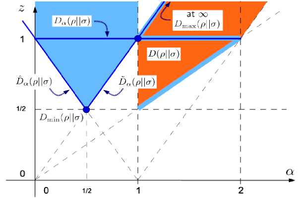
Figure A1.1. A schematic overview of the various relative entropies unified by the q-z-relative entropy is shown. [The blue region indicates the range of the parameters in which the DPI was proven, while the orange region indicates where it is just conjectured. To keep contact with the notation , the divergence functions S are indicated with the letter D, the parameter q is indicated with a, D ( pP|ct) is the von Neu mann relative entropy, Dmin is the logarithm of the fidelity and Dm:= inf {/: p < 2;^J].
Since we are interested in computing the metric tensors starting from this two-parameter family of two-point functions, it is convenient to consider the following regularization of the logarithm, the so-called q- logarithm:
log q p = — ( p'q - 1 ) with limlog q p = log p (A1.13) 1 - q q > 1
Moreover, inspired by Petz, we will consider a rescaling by a factor 1/ q . In this way, the resulting family of functions will be symmetric under the exchange of q ^ ( 1 - q ) . Let us denote the resulting two-point function with the same symbol of the q-z- RRE, that is:
S q , z ( P C ) =
q (q - 1)
f q 1 - q
1 - Tr c z p z к
z
(A1.14)
Since the analysis of the DPI involves only the trace functional, we are ensured that the DPI holds for the same range of parameters of the q-z-RRE. Moreover, in the limit z ^ 1, it is possible to recover the expression for the Tsallis relative entropy as z q (1 q)L in the limit z = q ^ 1, we recover the von Neumann relative entropy (A1.12) as in the limit z = q = □ , we recover the divergence function of the Bures metric tensor
1 - Tr ( p c )D
(A1.17)
2’2 z=q and finally, in the limit z = 1, q ^П , we recover the divergence function of the Wigner-Yanase metric tensor:
-
S 1 ( P к ) : = lim S q , z ( p к ) = SWY ( P к ) = 4 [ 1 - Tr ( P CD ) ] (AU8)
2,1 z = 1, q ^2
All these special cases belong to the range of parameters for which S is actually a quantum divergence function satisfying the DPI. Consequently, the family of associated quantum metric tensors satisfies the monotonicity property.
Appendix 2: Entropic-like uncertainty relations
The uncertainty principle is an essential feature of quantum mechanics, characterizing the experimental measurement incompatibility of non-commuting quantum mechanical observables in the preparation of quantum states. Heisenberg first introduced variance-based uncertainty. Later, Robertson proposed the well- known formula of the uncertainty relation, Var ( p, R ) Var ( p, S )> — |-rp[ R, S ]| , for arbitrary observa bles R and S, where [R, S] = RS — SR and Var (p, R) is the standard deviation of R. Schrodinger gave a further improved uncertainty relation:
where ^ R ^ = Tr ( p R ) , and { R , S } = RS + SR is anti-commutator. Since then many kinds of uncertainty relations have been presented. In addition to the uncertainty of the standard deviation, entropy can be used to quantify uncertainties. The first entropic uncertainty relation was given by Deutsch and was then improved by Maassen and Uffink:
where R = {| u} ^} and S = {| uk)} are two orthonormal bases on d-dimensional Hilbert space H, and H (R) = —^ z Pj log Pj (H (S) = — ^ , qk log qk) is the Shannon entropy of the probability distribution Pj = Uj |p|u^ (qk = (u|p|u}) for state p of H. The number c is the largest overlap among all cjk = |(и, |u)| between the projective measurements R and S. Berta et al. bridged the gap between cryptographic scenarios and the uncertainty principle and derived this landmark uncertainty relation for measure- ments R and S in the presence of quantum memory B:
H ( RB ) + H ( S|B ) > log,1 + H ( A\B ) where
H ( RB ) = H ( P„ ) — H ( P b ) is the conditional entropy with p^ = E. (| Uj } (u | ® Ip-. (| Uj ) Uj I ® I ) (similarly for H ( S| B ) ), and d is the dimension of the subsystem A . The term H ( ДБ ) = H ( pAB ) — H ( pB ) appearing on the right-hand side is related to the entanglement between the measured particle A and the quantum memory B . The bound of Berta et al. has been further improved. Moreover, there are also some uncertainty relations given by the generalized entropies, such as the Renyi entropy and the Tsallis entropy, and even more general entropies such as the ( h , Ф ) entropies. These uncertainty relations not only manifest the physical implications of the quantum world but also play roles in entanglement detection, quantum spin squeezing and quantum metrology.
An uncertainty relation based on Wigner -Yanase skew information I (p, H) has been obtained with quantum memory, where I (p, H ) = ^Tr
= Tr ( p H 2 ) - Tr ( ^J p H pHH ) quantifies the
degree of non-commutativity between a quantum state p and an observable H , which is reduced to the variance Var ( p , H ) when p is a pure state. In fact, the Wigner-Yanase skew information I ( p , H ) is generalized to Wigner–Yanase–Dyson skew information:
I a ( p , H ) = 1 Tr [ ( i [ pa , H ] )( i [ p1"" , H ] ) ] = Tr ( p H 2 ) - Tr ( pa H p'-“ H ) a e [ 0,1 ] . (A2.1)
Here theWigner-Yanase-Dyson skew information Ia ( p , H ) reduces to theWigner-Yanase skew information I ( p , H ) , when a =□ . The Wigner-Yanase-Dyson skew information Ia ( p , H ) reduces to the standard deviation Var ( p , H ) when p is a pure state. The convexity of Ia ( p , H ) with respect to p has been proven by Lieb. Kenjiro introduced another quantity:
where H = H — Tr ( p H ) I with I being the identity operator. For a quantum state r and observables R, S and 0 < a < 1 , the following inequality holds:
where Ua (p,R) = Ia (p, R) Ia (p, R) can be regarded as a kind of measure for quantum uncertainty. For a pure state, a standard deviation-based relation is recovered from Eq. (A2.3).
Let ф = |ф)(Ф I and ^ = |^)(^ | be the rank 1 spectral projectors of two non-degenerate observables R and S with the eigenvectors |ф) and |^ }, respectively. We can define U^a (P,Ф) = E Ua ( P,Фk ) = E 7I a (P,Фk ) I a ( P,Фk )Ua (p, ^ ) as the uncertainty of p associated to kk the projective measurement {ф } , and Ua (p,^) to \yk } .
Let p AB be a bipartite state on HA ® HB , where HA and HB denote the Hilbert space of subsystems A and B , respectively. Let V be any orthogonal basis space on HA and | ф ) be an orthogonal basis of HA . We define a quantum correlation of p AB as
Vk where the minimum is taken over all the orthogonal bases on HA , pA = TrBpAB . For any bipartite state pAB and any observable XA on HA , we have Ia (pAB, XA ® IB ) > Ia (pA, XA ) . Therefore, Da (pAB ) > 0 .
Furthermore, Da ( pAB ) = 0 when pAB is a classical quantum correlated state.
Da ( Pab ) has a measurement on subsystem A , which gives an explicit physical meaning: it is the minimal difference of incompatibility of the projective measurement on the bipartite state pAB and on the local reduced state pA . Da ( pAB ) quantifies the quantum correlations between the subsystems A and B . We have the following.
Theorem A2.1. Let pAB be a bipartite quantum state on HA ® HB and { ф } and {vk } be two sets of rank 1 projective measurements on H . Then
UN a ( P ab - Ф ® I ) UN . ( P ab V ® I ) > Z L p ( Ф к - V k ) + D a ( P ab ) (A2.5)
k
1 I \ H \ l Tr PA [Ф V ]|2
where La , p a ф к - V k ) = a ( 1 - a ) , .
41 a ( P a , ф к ) I a ( P a - V k )
Theorem A2.1 gives a product form of the uncertainty relation. Comparing the results (Eq. (A2.3)) without quantum memory with those (Eq. (A2.5)) with quantum memory, one finds that if the observables A and B satisfy [ A , B ] = 0 , the bound is trivial in Eq.(A2.3), while in Eq. (A2.5), even if the projective measurements ф and Vk satisfy [фк Vk ] = 0 , that is, La p (фк Vk ) = 0 , Da ( pAB ) may still not be trivial because of correlations between the system and the quantum memory.
Corresponding to the product form of the uncertainty relation, we can also derive the sum form of the uncertainty relation:
Theorem A2.2. Let pAB be a quantum state on HA ® HB and { ф } and { v } be two sets of rank 1 projective measurements on H . Then
k
From Theorems A2.1 and A2.2, we obtain uncertainty relations in the form of the product and sum of skew information, which are different from the uncertainty, which only deals with the single partite state. However, we treat the bipartite case with quantum memory B. It is shown that the lower bound contains two terms: one is the quantum correlation Da (pAB ) , and the other is ^La p(фк ,v ) which characterizes the k degree of compatibility of the two measurements, just as for the meaning of log2 — in the entropy uncertain-c ty relation.
For the Shannon entropy, Renyi entropy, Tsallis entropy, ( h , Ф ) entropies and Wigner-Yanase skew information, theWigner-Yanase-Dyson skew information characterizes a special kind of information of a system or measurement outcomes, which needs to satisfy certain restrictions for given measurements and correlations between the system and the memory. Different a parameter values give rise to different kinds of information.
The uncertainty relations both in product and summation forms in terms of the Wigner-Yanase-Dyson skew information with quantum memory have investigated. It has been shown that the lower bounds contain two terms: one is the quantum correlation Da (pAB) , and the other is ^La рффк,Vk ), which characterizes k the degree of compatibility of the two measurements.
References Basic relations of quantum information theory. Pt 2: classical, quantum and total correlations in quantum state - measure of quantum accessible information
- Килин С.Я. Квантовая информация // УФН. - 1999. - Т. 169. - № 5.
- EDN: MQDTZJ
- Холево А.С. Введение в квантовую теорию информации. - М.: 2002.
- Keyl M. Fundamentals of quantum information theory // Physical Reports. - 2002. - V. 369. - № 5.
- EDN: MCDGND
- Cerf N.J., Adami C. Negative entropy and information in quantum mechanics. // Physical Review Letters. - 1997. - V. 79. - № 26.
- Horodecki M., Oppenheim J., Winter A. Partial quantum information. // Nature. - 2005. - V. 436. - № 7051.
