Bearing Health Assessment Using Time Domain Analysis of Vibration Signal

Published Online June 2020 in MECS DOI: 10.5815/ijigsp.2020.03.04

Induction motor is an electromechanical device that converts alternating electrical energy into mechanical energy with the help of stator windings, rotor bars, and bearings. The mechanical power generated over rotor bars, transfers to external load with the help of rotor shaft and bearings. For the smooth movement of the prime mover, the bearing used in it should be healthy. From the survey reports of various agencies on percentage failure components of induction motor, it has been estimated that approximate 30-40% failures are related to stator windings, 40-50% failures are associated to bearings, 510% failures are associated with rotor bars, and 10-12% failures are related with other components of induction motor [1, 2]. Thus, bearing faults are the most frequent occurring defect in an induction motor.

Bearing defects may broadly be classified as distributed and single point defects [3]. A distributed defect incorporates surface roughness, waviness, misaligned races, and off-size rolling elements, while localized defect includes pits, cracks, and spalls on races or rolling surfaces of bearing. The major cause of rolling element bearing failure is the spalling on the rolling elements or races [4]. If these faults are not detected and diagnosed in an early stage then these may cause complete failure of machine that may result into huge economical loss, complete shutdown of the plant, and personal casualties.

Bearing defects may be detected using acoustic analysis, temperature monitoring, oil analysis, stator current and vibration analysis [5, 6, 7, 8, 9]. B. V. Hecke et al., [7] proposed a method using acoustic emission analysis to identify bearing deficiency of motor running at very low speed. Acoustic and noise analysis is an effective method to identify mechanical defects of IM, however the accuracy of fault prediction depends on the sound stress and its concentration. The temperature monitoring can be performed by using resistance temperature detector (RTD), thermocouples, infrared temperature detector, embedded temperature sensors in IM housing and thermographic cameras [8]. However, this method is not able to identify the localized defect in its very early stage, and require costly instruments to process the temperature variation to identify the IM faults. In wear debris analysis method, the debris particles generated in machine are assessed in terms of type, size, composition, mass and morphology [9]. The variations in any one of these factors are used as index parameter to determine the mechanical faults. However, it is generally offline process, sensors used are costly and chemical analysis of oil is time consuming [10]. Stator current and vibration signals are the most significant parameters to detect bearing defects [11]. The stator current based bearing fault monitoring will be effective only for the faults having low characteristic frequencies [12]. In contrast, vibration signal is widely applicable and robust parameter to detect bearing defects at any operating conditions [13]. The localized defect produces a progression of effect vibrations each time, running roller passes over the surface of deformities. Hence, through the utilization of some matured analysis techniques of the vibration signal, vital and rich fault diagnostic information about bearing can be obtained.

Time-domain, frequency-domain, and time-frequency domain based feature analysis of vibration signals are some common techniques to analyze bearing defects. Fast Fourier transform (FFT) is the basic frequency analysis technique to extract fault frequencies present in vibration signal [14]. Due to the non-stationary nature of vibration signal, time-frequency based methods like short-time-Fourier transform (STFT), wavelet transform (WT), and adaptive time-frequency based methods may play a significant role in extracting the bearing fault information [15, 16, 17, 18]. However, these techniques require complex mathematical model and large processing time to analyze the signals [18]. Therefore, authors of this manuscript proposed a simple computation approach utilizing time-domain features of vibration signal to analyze bearing defects.

Few authors have also extracted time-domain features of vibration signal like Peak value, mean value, RMS value, zero crossings, crest factor, standard deviation, skewness, and kurtosis, etc. to identify bearing defects [19, 20, 21, 22]. However, only comparing magnitudes of these time-domain features are not always effective to identify bearing defects [23]. In recent decade, artificial intelligence (AI) techniques are widely being used to diagnose bearing defects due to its robustness toward noise and automatic decision capabilities [23, 24, 25]. J. B. Ali et al., [26] have incorporated statistical features of vibration signal and ANN technique to identify bearing defects. In this method, empirical mode decomposition

(EMD) energy entropy based statistical features were extracted from vibration signal. B. Nayana et al., [27] have utilized time-domain features like Mean, Absolute Value (MAV), Simple sign Integral (SSI), Willison Amplitude (WAMP), Zero Crossing (ZC) and Slope Sign Change (SSC) of vibration signal along with feature reduction methods and support vector machine (SVM) to identify bearing defects. Few researchers have also focused on incorporating hybrid intelligent techniques like Adaptive Neuro-Fuzzy Inference System (ANFIS) [28], Adaptive Fuzzy-C Mean clustering [29] etc. with statistical features of vibration signal to identify bearing defects. However, the accuracy of fault prediction algorithm is generally depending upon the number and discriminating potential of the features extracted from characteristic signals [30, 31].

In this perspective, this manuscript proposed a novel statistical time-domain approach utilizing vibration signal to diagnose rolling element bearing defects. For this, sixtime domain features (TDFs) namely Mean Value (µ), Peak value, Root Mean Square (RMS), Crest Factor (CRF), Skewness (SKW) and Kurtosis (K) were extracted from standard vibration database due to their abilities to reflect the variations in time series signal. The vibration databases were taken from the Case Western Reserve University (CWRU) website as healthy, inner raceway (IR) and ball (BB) defects of bearing at fault levels 7 mils, 14 mils, 21 mils, and 28mils and at mechanical loads 0HP, 1HP, 2HP, and 3HP. For better analysis, extracted TDFs were processed using three statistical methods to validate the effectiveness of these TDFs in identifying bearing defects. In the first approach, the mean and standard deviation (σ) of each considered TDF was computed and analyzed to study the bearing defects. This study provides an easy way to analyze the variations in TDFs corresponding to different health conditions of bearing. In the second scheme, the box or whisker plot method was applied to visualize the variation of each TDF in terms of median and Inter Quartile Range (IQR) value. This scheme provides a more analytical approach to diagnose bearing defects. In the third scheme, a new index parameter named as Bearing Fault Index based on Time Domain Features (BFIT) was measured and compared to investigate bearing defects. This parameter predicts the bearing defects based on the mean of all considered TDF. The results of the proposed scheme have shown that analysis of TDFs of vibration signal is simple and reliable to diagnose bearing defects.

The rest of this manuscript is organized as follows. The description of the test rig and vibration database has been reported in section II. Section III illustrates the interpretation of considered time-domain features (TDF) like mean value, peak, RMS, crest factor, kurtosis, and skewness, used to process vibration signal. It also includes the comparative analysis in variation of considered TDF to identify bearing defects. Section IV consists of results and discussion of statistical analysis of considered TDF in terms of mean and standard deviation analysis, box plot analysis, and BFIT analysis to identify bearing defects. The conclusion of the work is presented in section V.

• II.    Proposed Method

As mentioned in the previous section, the purpose of this work is to identify bearing defects using timedomain features of the vibration signal. Fig. 1 presents a block diagram of the proposed fault detection process. To validate the proposed method thirty-six standard databases of vibration signals were collected from publicly available datacenter website of Case Western

Reserve University [32, 33]. The proposed method includes the computation of six time-domain features namely Mean Value (µ), Peak value, Root Mean Square (RMS), Crest Factor (CRF), Skewness (SKW) and Kurtosis (K) of segmented vibration datasets and process them using statistical methods as “mean±σ” analysis, and box plot analysis to analyze bearing defects. For a better analysis of bearing defects, a new index parameter termed as bearing fault index (BFIT) was also introduced that was computed by the mean of all considered TDFs. The next section will describe the vibration databases used for bearing faults diagnosis.

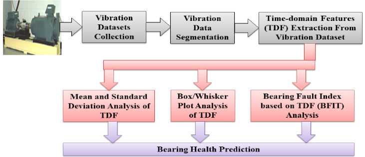
Fig.1. Methodology to detect bearing defects using time domain features of vibration signal

• A.    Vibration Database

  In this manuscript, vibration signal is used as characteristic parameter due to its direct relationship with the bearing defects. For this, the standard vibration databases were taken from the publicly available datacenter website of Case Western Reserve University (CWRU) [32, 33]. The SKF-6205 ball bearing assembled at drive end side of 2HP reliance made induction motor was seeded faults using electro-discharge machining (EDM) technology with depth of 7 mils (0.01778mm), 14 mils (0.03556mm), 21 mils (0.05334mm), and 28mils ( 0.07112mm) at the inner raceway, and rolling ball. Each of the vibration databases were acquired at a 12 kHz sampling rate using a 16 channel DATA recorder for 10 seconds duration i.e. 120000 samples in each dataset. The vibration datasets are derived for bearing conditions namely no fault (NF), inner raceway defects (IR) and ball defects (BB) at different fault depths for motor loads 0HP, 1HP, 2HP, and 3HP. Thus, total thirty-six vibration databases have been recorded that are reported in Table 1 . Dataset NF has four databases namely NF_0, NF_1, NF_2, and NF_3 that are derived at motor loads 0HP, 1HP, 2HP and 3HP respectively. Datasets of inner raceway defects like IR_a, IR_b, IR_c, and IR_d, and ball defects like BB_a, BB_b, BB_c, and BB_d are acquired at fault depths of 7 mils, 14 mils, 21 mils, and 28 mils respectively. Each of these datasets was also recorded at motor loads 0HP, 1HP, 2HP and 3HP. The vibration datasets were symbolized as NF_load, IR_fault-diameter_load, BB_fault-diameter_load. The time-

• domain waveform of vibration datasets NF_0, IR_a_0, and BB_a_0 are shown in Fig.2 for duration of 1second. To analyze even small variations in the vibration signal, the samples of each database were segmented into 100 segments of 1,200 samples each.

Table 1. Considered vibration datasets to study bearing health conditions

Bearing Health Status		Datas et	0 HP	1 HP	2 HP	3 HP
	Fault Diamet er
Health y	NA	NF	NF_0	NF_1	NF_2	NF_3
	7 mils	IR_a	IR_a_ 0	IR_a _1	IR_a _2	IR_a 3
Inner Racew	14 mils	IR_b	IR_b_ 0	IR_b _1	IR_b _2	IR_b _3
ay Defects	21 mils	IR_c	IR_c_ 0	IR_c _1	IR_c _2	IR_c _3
	28 mils	IR_d	IR_d _0	IR_d _1	IR_d_ 2	IR_d_ 3
	7 mils	BB_a	BB_a_ 0	BB_a_ 1	BB_a_ 2	BB_a_ 3
Ball	14 mils	BB_b	BB_b _0	BB_b _1	BB_b _2	BB_b _3
Defects	21 mils	BB_c	BB_c_ 0	BB_c_ 1	BB_c_ 2	BB_c_ 3
	28 mils	BB_d	BB_d _0	BB_d _1	BB_d _2	BB_d _3

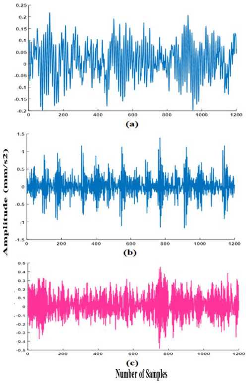
Fig. 2. Time waveform of the segmented raw data of vibration dataset (a) NF_0 (b) IR_a_0 (c) BB_a_0

• B.    Feature Extraction

As we know that the amplitude of the vibration signal extracted from bearings of induction motor is the function of time, so time-domain analysis of vibration signal can provide significant information about bearing health conditions. In this work, six time-domain features (TDFs) namely mean value (μ), peak value (peak), root mean square (RMS), crest factor (CRF), kurtosis (K), and skewness (SKW) were computed to analyze bearing defects.

Assume that X j is the segmented database of vibration signal, where j = 1,2, 3.......n , and n represents the length of the dataset, and then the TDFs of segmented vibration database are computed using equation (1) to equation (6).

Mean Value (μ): It represents the average value of the sampled dataset. It is used to determine the distribution symmetry of data over reference value. The mean value of a dataset can be calculated using equation (1).

M =

2 x , j = 1

n

Peak Value ( Peak ): It denotes the maximum value of the amplitude of dataset. Mathematically, it is represented by equation (2).

peak = max x

Root Mean Square (RMS) : It articulates the energy content of the sampled data signal. RMS value is directly related to the energy of the signal so it may have useful information about the destruction of the signal. It is expressed by equation (3).

RMS

Crest Factor (CRF) : It is the ratio of peak value to the RMS value of the signal. It represents how extreme the peaks are in datasets. The CRF near to 1 represents a lower spiky signal. The CRF is computed using equation (4).

peak

CRF = ---

RMS

Kurtosis (K): It indicates whether the signal distribution is flat or peaked. Low kurtosis value represents that the signal is flat whether high kurtosis value represents that the signal is peaky. Equation (5) shows the mathematical expression of kurtosis.

K =

n

¹ 2 ( x — M ) 4 ⁿ          j

4 а

Where а = deviation value

1 ⁿ

2 ^{( x} - m ⁾² n M ^j

represents standard

Skewness (SKW): It indicates asymmetric probability distribution of sampled data about its mean value. Negative valued skewness indicates that data is skewed toward left whether positive value skewness represents that the data is skewed towards the right. The skewness factor of signal is computed by using equation (6).

1 ⁿ

2 ( x - M )

nj

SKW = —j= ------- (6)

а

• C.    Feature Analysis

The TDFs of segmented vibration databases were further processed using three statistical methods termed as mean and standard deviation (mean±σ) analysis, box plot analysis, and a new proposed method bearing fault index (BFIT) analysis. These methods were applied to analyze the variations in TDFs for better demarcation of bearing conditions.

• i.    Mean And Standard Deviation Analysis

In this analysis, the mean and standard deviation of each TDF were computed from segmented database of vibration signal. The computed values of mean±σ of each database were compared and analyzed to study the variation in its magnitude to demarcate the different health conditions of bearing.

• ii.    Box Plot Analysis

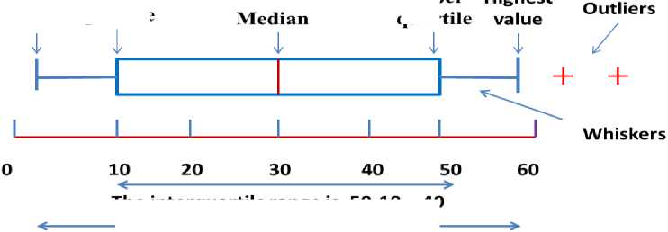
In descriptive statistics, a box or whisker plot is a pictorial representation of the distribution of numerical data through quartiles, maximum and minimum. Quartiles are used to split an ordered dataset into four parts. These quartiles are termed as lower quartile (Q1), middle quartile or median (Q2) and upper quartile (Q3). The difference of upper quartile to lower quartile is known as Inter Quartile Range (IQR). The highest value of dataset that is inside 1.5 times of the IQR above upper quartile is termed as the maximum value and minimum value that lies within the range of 1.5 times the IQR to below lower quartile is known as minimum value. The width of the box represents the sample size of the data. Any value of data that is higher than maximum value and lower than minimum value is known as outliers that are represented by a cross with a red color. The difference between maximum to the minimum value of data is characterized as DM. the whiskers are represented by green lines. A sample box plot having all related terms is shown in Fig.3.

Lowest Lower value quartile

The interquartile range is 50-10 = 40

The range is 58-2 = 56

Fig. 3. Graphical representation of box or whisker plot and their parameters indicated by blue and red line

Let Q1- lower quartile , Q2- median , Q3- upper quartile , then

The interquartile range, iqr = Q₃ - q_x

Lowest value: The minimum value of dataset that

• > Q i - 1.5 x IQR

Highest value: The maximum value of dataset that is <  Q ₃ + 1.5 x IQR

• iii.    Bearing Fault Index

There is need to determine a unique and robust fault index parameter that can predict the bearing health conditions with more reliable results. For this, a new index parameter was measured that is termed as Bearing Fault Index (BFIT). This parameter predicts the bearing defects based on the mean of all considered TDF at all machine loads. This parameter will be very much helpful in predicting the health conditions of bearing as it considered all operating conditions of machine. Mathematically it is represented as equation (7).

BFIT = mean | д , peak , RMS , CRF , K , SKW |    (7)

• III.    Results And Discussion

This section of the manuscript presents the brief discussion about the results of proposed statistical analysis of TDFs of vibration dataset to identifying inner raceway and ball defects of rolling element bearing. In this manuscript, two most versatile statistical approach as mean±σ analysis, and box plot analysis along with a novel proposed statistical parameter as BFIT were investigated for better diagnostic results. The results of each statistical analysis were presented separately.

• A.    Time Domain Feature Extraction

  In this analysis, each vibration dataset is processed using MATLAB 2017a software to compute the considered TDFs. Fig.4 represents the variation of considered TDF of vibration datasets related to bearing health conditions as healthy, inner raceway and ball bearing defects at motor loads 0HP, 1HP, 2HP, and 3HP. The x-axis of figures represents the number of segments of vibration datasets at different health conditions of bearing. The segments 1 to 100 indicate variation of NF,

101 to 200 variation of IR_a, 201 to 300 variation of IR_b, 301 to 400 variation of IR_c, 401 to 500 variation of IR_d, 501 to 600 variation of BB_a, 601 to 700 variation of BB_b, 701 to 800 variation of BB_c and 801 to 900 represents variation of BB_d bearing health condition.

Fig.4 (a) represents the variation of the values of the mean feature of segmented vibration datasets. The results of the figure reflect that the value of feature decreases with an increase in inner raceway fault severities of bearing on all considered load except 0HP. This figure also reflects that the value of healthy bearing is higher than bearing having ball defects except at 3HP load. The value of the vibration signal related to ball-bearing defects suddenly increases at 3HP load. These values allude that the value of NF bearing is higher than the faulty bearing.

The variation of peak value at different bearing conditions is shown in Fig.4 (b). This figure depicts that peak value for NF bearing is less than 0.3 while bearing having IR fault is higher than 1 and ball defect is higher than 0.3. This value increases with an increase in IR fault severities, while it is almost unaffected with an increase in ball fault severities. From the obtained figure, it has also observed that the peak value of vibrations suddenly increases in induction motor having ball bearing defects and operated at 3HP load. Thus from peak value, it is concluded that the induction motor generates more peaked vibration having a defective bearing.

The RMS value of the segmented vibration dataset is depicted in Fig.4 (c). The result of this figure demonstrates that RMS value for NF bearing is around 0.1, for IR_a is near to 0.3, IR_b is around 0.2, IR_c is near to 0.5, IR_d is near to 0.14 and for all BB defects are near to 0.14. The figure indicates that the RMS value of vibration datasets for induction motor having healthy bearing is near to 0.1 and defective bearing with IR fault and BB fault is higher than 0.1. The figure also depicts that induction motor having BB defects and operating at 3HP load shows a very high value of RMS. Thus from graphical representation, it is concluded that the RMS value of defective bearing is higher than 0.1 while for healthy bearing it is less than 0.1.

The variation of the CRF feature is shown in Fig.4 (d). It depicts that this value for NF bearing is around 3.12 and increases with IR fault severities. Its value for IR_a has fluctuated near 4.8; IR_b is varying around 8.15, for IR_c varies near to 5.66 and for IR_d decreases near to 4.3 at 0HP load. The variation in CRF value of vibration data segments for ball defects BB_a at 0HP load is near to 3.39 and it is almost constant with an increase in ball defect severities. The figure also depicts that CRF value increases with an increase in motor load.

Fig.4 (e) reflects the variation of kurtosis (K) of bearing vibration data segments. The results of the figure show that its value is near to 2.75 for NF bearing and around 5.38 for IR_a, near 21.65 for IR_b and around 7.29 for IR_c and 5.26 for IR_d bearing defects. The results of this figure reveal that the value of K increases with an increase in bearing fault then decreases. The figure also illustrates that the values of K for ball defective bearings are almost constant and varied near to 2.9. However, from the figure, it is concluded that the value of K for defective bearings is always higher than the healthy bearing.

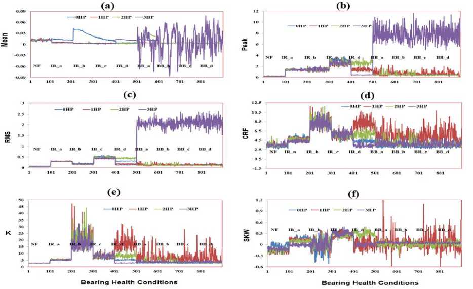
Fig.4. Representation of (a) mean (µ) (b) Peak (c) RMS (d) Crest Factor (CRF) (e) Skewness (SKW) (f) Kurtosis (K) time-domain features on different loads as 0HP, 1HP, 2HP and 3HP

Fig.4 (f) shows the variation of skewness (SKW) and this value increases with a rise in IR fault levels. However, this value decreases above 21mils of IR fault. It eludes that at a severe stage of IR fault, the SKW feature creates a problem in predicting the faults. The figure also shows that the SKW feature for bearing having ball fault is higher than the healthy bearing. Thus from the time-domain representation of TDF, it is concluded that TDF is effective at initial stage faults while it became ineffective at an extreme level of defects. These values have been verified with the results of research work published by Fu et al., [29]. For more effective analysis of bearing faults using considered TDF of the vibration signal, mean and standard deviation of each TDF was determined and analyzed.

• B.    Mean And Standard Deviation Analysis Of Features

In this study, mean and standard deviation (Mean ± σ) of all six considered TDF of segmented datasets were computed and results are shown in Table 2 . The results of Table 2 allude that the μ value of NF bearing is approximately the same as the μ value of IR_a, IR_b, IR_c and BB_a faults at 0HP load.

Table 2. Mean ±σ of TDF of vibration datasets corresponding to different bearing conditions

	Load	0HP	1HP	2HP	3HP
Features	Bearing Conditions	Mean ± σ	Mean ± σ	Mean ± σ	Mean ± σ
	NF	0.013 ± 0.001	0.013 ± 0.002	0.012 ± 0.002	0.012 ± 0.002
	IR_a	0.013 ± 0.001	0.006 ± 0.001	0.005 ± 0	0.005 ± 0.001
	IR_b	0.012 ± 0.009	0.004 ± 0	0.004 ± 0.001	0.003 ± 0
	IR_c	0.014 ± 0.003	0.003 ± 0.001	0.003 ± 0.001	0.003 ± 0.001
µ	IR_d	0.005 ± 0.001	0.003 ± 0	0.003 ± 0.001	0.013 ± 0.002
	BB_a	0.013 ± 0.002	0.005 ± 0	0.021 ± 0.01	0.005 ± 0.025
	BB_b	0.004 ± 0	0.005 ± 0	0.004 ± 0	0.009 ± 0.038
	BB_c	0.005 ± 0	0.005 ± 0.001	0.005 ± 0	0 ± 0.027
	BB_d	0.004 ± 0	0.005 ± 0	0.004 ± 0	0.019 ± 0.027
	NF	0.233 ± 0.019	0.22 ± 0.019	0.216 ± 0.022	0.228 ± 0.02
	IR_a	1.427 ± 0.128	1.393 ± 0.106	1.377 ± 0.104	1.335 ± 0.098
	IR_b	1.576 ± 0.165	1.334 ± 0.225	1.33 ± 0.209	1.404 ± 0.249
	IR_c	2.945 ± 0.4	2.436 ± 0.314	2.647 ± 0.304	2.59 ± 0.314
Peak	IR_d	1.335 ± 0.098	1.404 ± 0.249	2.59 ± 0.314	0.456 ± 0.05
	BB_a	0.456 ± 0.05	0.775 ± 0.481	0.539 ± 0.243	7.934 ± 1.215
	BB_b	0.453 ± 0.047	0.708 ± 0.24	0.504 ± 0.273	7.629 ± 1.301
	BB_c	0.466 ± 0.046	0.737 ± 0.332	0.38 ± 0.051	7.799 ± 1.188
	BB_d	0.495 ± 0.053	0.719 ± 0.386	0.401 ± 0.041	7.925 ± 1.377
	NF	0.074 ± 0.002	0.066 ± 0.001	0.064 ± 0.001	0.066 ± 0.001
	IR_a	0.291 ± 0.005	0.293 ± 0.004	0.299 ± 0.005	0.314 ± 0.008
	IR_b	0.197 ± 0.013	0.165 ± 0.015	0.163 ± 0.011	0.18 ± 0.012
RMS	IR_c	0.525 ± 0.023	0.441 ± 0.02	0.488 ± 0.027	0.448 ± 0.023
	IR_d	0.314 ± 0.008	0.18 ± 0.012	0.448 ± 0.023	0.139 ± 0.007
	BB_a	0.139 ± 0.007	0.142 ± 0.055	0.131 ± 0.036	2.072 ± 0.144
	BB_b	0.139 ± 0.005	0.137 ± 0.032	0.123 ± 0.038	2.022 ± 0.175
	BB_c	0.147 ± 0.006	0.14 ± 0.032	0.107 ± 0.005	2.138 ± 0.186
	BB_d	0.153 ± 0.007	0.129 ± 0.036	0.118 ± 0.004	2.131 ± 0.25

CRF

SKW

NF	3.123 ± 0.22	3.198 ± 0.291	3.175 ± 0.202	3.163 ± 0.206
IR_a	4.9 ± 0.435	4.762 ± 0.352	4.61 ± 0.328	4.306 ± 0.249
IR_b	8.158 ± 0.766	8.516 ± 1.032	8.483 ± 1.061	8.055 ± 1.094
IR_c	5.6 ± 0.63	5.517 ± 0.642	5.44 ± 0.544	5.782 ± 0.656
IR_d	4.306 ± 0.249	8.055 ± 1.094	5.782 ± 0.656	3.896 ± 0.34
BB_a	3.496 ± 0.34	5.302 ± 1.451	4.087 ± 0.586	3.84 ± 0.565
BB_b	3.571 ± 0.307	5.285 ± 0.936	4.05 ± 0.822	3.782 ± 0.522
BB_c	3.542 ± 0.3	5.358 ± 1.369	3.664 ± 0.34	3.668 ± 0.503
BB_d	3.618 ± 0.339	5.516 ± 1.507	3.791 ± 0.288	3.74 ± 0.504
NF	2.754 ± 0.121	2.921 ± 0.11	2.918 ± 0.091	2.951 ± 0.093
IR_a	5.385 ± 0.363	5.529 ± 0.316	5.548 ± 0.269	5.262 ± 0.236
IR_b	21.658 ± 3.825	21.062 ± 6.014	21.032 ± 5.481	17.536 ± 4.665
IR_c	7.291 ± 1.232	7.574 ± 1.308	7.93 ± 0.96	8.232 ± 1.367
IR_d	5.262 ± 0.236	17.536 ± 4.665	8.232 ± 1.367	3.151 ± 0.196
BB_a	2.951 ± 0.196	6.958 ± 4.873	3.828 ± 0.897	3.831 ± 0.595
BB_b	2.941 ± 0.187	6.44 ± 2.294	3.923 ± 1.458	3.782 ± 0.627
BB_c	2.943 ± 0.187	6.494 ± 3.688	3.247 ± 0.258	3.684 ± 0.585
BB_d	2.973 ± 0.217	7.055 ± 4.222	3.082 ± 0.179	3.733 ± 0.536
NF	-0.035 ± 0.057	-0.173 ± 0.046	-0.167 ± 0.048	-0.128 ± 0.045
IR_a	0.164 ± 0.049	0.13 ± 0.04	0.09 ± 0.035	0.013 ± 0.038
IR_b	0.061 ± 0.174	0.004 ± 0.149	0.025 ± 0.145	0.026 ± 0.153
IR_c	0.303 ± 0.054	0.257 ± 0.066	0.249 ± 0.055	0.304 ± 0.067
IR_d	0.053 ± 0.038	0.026 ± 0.153	0.304 ± 0.067	0.009 ± 0.037
BB_a	-0.001 ± 0.037	0.067 ± 0.225	0.002 ± 0.055	0.055 ± 0.02
BB_b	0.007 ± 0.033	0.014 ± 0.097	-0.001 ± 0.069	0.047 ± 0.018
BB_c	0.026 ± 0.036	0.081 ± 0.216	0.001 ± 0.056	0.041 ± 0.016
BB_d	0.02 ± 0.036	0.028 ± 0.229	0.026 ± 0.052	0.041 ± 0.015

While this value decreased from 0.013 to 0.012 for NF, 0.013 to 0.005 for IR_a, 0.012 to 0.003 for IR_b, 0.014 to 0.003 for IR_c and 0.013 to 0.005 for BB_a condition if load increasing from 0HP to 3HP. For other bearing conditions like IR_d, BB_b, BB_c, and BB_d, μ value is approximately the same at increasing load except for 3HP load. The result also indicated that у is very low for each dataset except at 3HP load. It indicates that vibration fluctuation is higher at the 3HP load. Thus from the ц study of the table, it is concluded that the mean vibration signal decreases with an increase in defect levels and approximates the same with the load. From the results of mean ± 7 analysis of peak feature as shown in Table 2, the mean value of peak feature for NF bearing is<1 while for IR fault is >1 even increasing the load. The у value of the peak for IR fault is also higher than NF bearing. For BB bearing the value of mean and σ, both are higher than NF bearing. Thus from the results of the peak of the table, it is concluded that the amplitude, as well as variation in peak, is very high in faulty bearing in comparison to the healthy bearing. The mean ±у analysis of RMS feature as shown in the table reflects that the mean of RMS value for NF bearing is 0.074 on 0HP and 0.066 on other considered loads which are<0.1, while this value is >0.1 for faulty bearing. The у value of RMS also indicates that it is almost double for faulty bearing in comparison to NF bearing. The results of Table 2 also show that the mean of CRF value for NF bearing is < 3.2 while it is >3.5 for IR and BB bearing. The у analysis of CRF also shows that it is higher at the faulty bearing. The value of the mean of kurtosis (K) for NF bearing varies from 2.754 to 2.951 while for IR_a varies from 5.385 to 5.262, IR_b varies from 21.658 to 17.53, IR_c varies from 7.291 to 8.232 and for IR_d varies from 3.151 to 17.536 on considered loads. The K values for BB_a varies from 2.951 to 6.958, BB_b varies from 2.941 to 6.44, BB_c varies from 2.943 to 6.494 and BB_d varies from 2.973 to 7.055. These values indicate that K is highest at 1HP load. Thus form the table, it is concluded that K value for the faulty bearing is higher than NF bearing. The SKW values for NF bearing are-0.035, -0.173, -0.167 and -0.128 at 0HP, 1HP, 2HP and 3HP load while SKW for IR bearing varies from 0.009 to 0.304 and for BB bearing, it varies from -0.001 to 0.081for loads varies from 0HP to 3HP. These values reflect that the skewness is almost negative for NF bearing and positive for faulty bearing on considered load.

• C.    Box Plot Analysis Of Features

For more accurate analysis for bearing defects, the box/whisker plots of considered TDF were analyzed. The box plot splits the sampled datasets in terms of median, and IQR value. The red horizontal line represents the median value of the sample, and difference between 3rd to 1st quartile of sample represents interquartile range (IQR). The results of box plot of individual TDFs were investigated separately.

The box plots of the mean feature of vibration signal for different bearing health conditions and machine operating loads are represented in Fig.5 . The box plot of Fig.5 (a) demonstrates that IQR and median parameter of µ time-domain feature at 0HP load increases with an increase in inner race bearing fault up to IR_b then continuously decreases. In contrast, Fig.5 (b), (c) and (d) show that the median and IQR of the mean feature of healthy bearing is higher than faulty bearing with IR defects. The results of the figure also show that the median and IQR of the mean feature of healthy bearing is higher than bearing having ball defects except at 3HP load. It indicates that ball bearing defects can easily be identified using a box plot analysis of mean feature under rated IM loads. Thus from box plot representation of a mean feature of the vibration signal, it can be concluded that the median of the mean for healthy bearing remains near to 0.012 while for IR bearing about 0.001 except 0HP load and for BB defects remains below 0.006 except 3HP load.

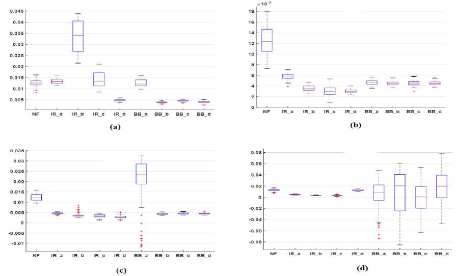
Fig.5. Box/whisker plot representation of the μ feature of different vibration datasets at machine loads (a) 0HP (b) 1HP (c) 2HP (d) 3HP

Fig.6 represents the box plot analysis of peak feature of vibration datasets at different bearing health conditions and loads. From the figure, it is noticeable that the median and IQR value increased with the inner raceway fault level up to level 21mils and then decreases. It indicates that the peak feature is more convenient to detect IR faults in its early stage. Fig.6 depicts that the median value of peak feature for the healthy bearing is less than 0.2 while for inner raceway defect higher than 0.2 and ball bearing defect greater than 0.4. So from box plot analysis of peak feature, bearing faults can easily be detected with higher accuracy. Thus from the box plot analysis of peak feature, it is concluded that this feature is more accurate than the mean feature in detecting bearing defects.

Fig.6. Box/whisker plot representation of the max feature of different vibration datasets at machine loads (a) 0HP (b) 1HP (c) 2HP (d) 3HP

The box plot analysis of RMS features of vibration datasets is shown in Fig.7. The figure signifies that the median and IQR value of RMS features related to IR and BB defects are almost double to the healthy bearing. The median value for the healthy bearing is near to 0.07 while for inner raceway fault it is larger than 0.15 and ball defects higher than 0.13. The figure also demonstrates that the median and IQR of RMS feature fluctuates with IR defects while remains almost constant at BB defects.

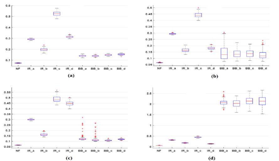
Fig.7. Box/whisker plot representation of the RMS feature of different vibration datasets at machine loads (a) 0HP (b) 1HP (c) 2HP (d) 3HP

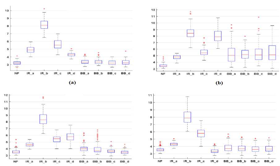
Fig.8 demonstrates the box plot analysis of the CRF feature. The figure demonstrates that the value of IQR rises with increased severity of defects. The median value of the CRF feature in the condition of healthy bearing becomes less than 3.5 while in the case of inner race defect of bearing it is more than 4 except at 3HP load. It depicts that IR faults can easily be identified using the CRF feature under full load conditions. While in the case of ball defects of bearing, a box plot of the CRF feature is not able to differentiate it from the healthy bearing. Normally, if its value ranges from 3 to 3.5 then a ball bearing defect is likely to occur.

(C)                                                                (d)

Fig.8. Box/whisker plot representation of the CRF feature of different vibration datasets at machine loads (a) 0HP (b) 1HP (c) 2HP (d) 3HP

The box plot of the kurtosis feature (K) is shown in Fig.9. The box plot findings show that the median of the K function is approximately 2.5 for NF bearing, which ranges from 5 to 20 for inner raceway defects under full load circumstances. The median of K feature initially rises to 22 with an increase in IR fault levels (up to 14mils) then starts a decrease. Box plot findings also show that the median of K features with ball defects is greater than that of NF bearing. Initially, the median of K features increases up 22 with an increase in IR fault levels (up to 14mils) then decreases. The results of the box plot also demonstrate that the median of K features with BB defects is higher than NF bearing. In spite of the above, the box plot representations of K feature of faulty bearing have several outliers while NF bearing has null outliers. The outliers represent the fluctuations of vibration signals in the defective bearing.

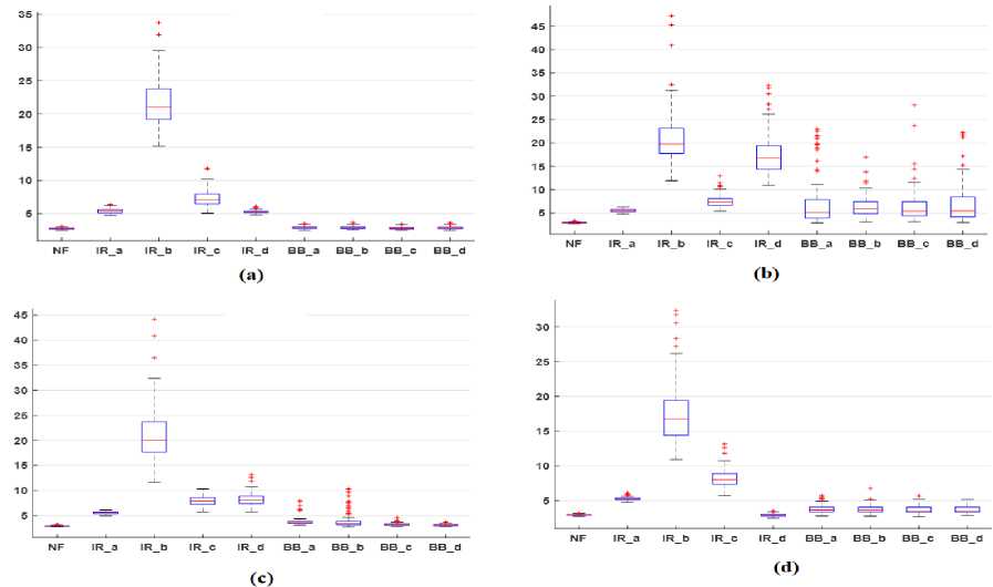
Fig.9. Box plot representation of the kurtosis (K) feature of different vibration datasets at machine loads (a) 0HP (b) 1HP (c) 2HP (d) 3HP

Fig.10 (a), (b), (c) and (d) demonstrate the box plot analysis of skewness (SKW) feature at operating loads 0HP, 1HP, 2HP and 3HP respectively. The results of the plot demonstrate that in the case of healthy bearing the median of SKW features is negative while in the case of faulty bearing it is almost positive. From Fig.10, it has also been observed that the median of faulty bearing is higher than the healthy bearing. Figure results also show that the median of SKW feature of BB fault is almost constant at different loads and higher than NF bearing.

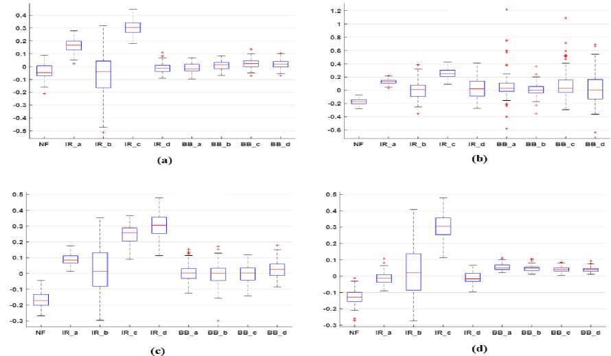
Fig.10. Box/whisker plot representation of the Skewness feature of different vibration datasets at machine loads (a) 0HP (b) 1HP (c) 2HP (d) 3HP

The results of box plot analysis of TDFs are summarized as:

• •    Mean feature is not much effective in differentiating bearing health conditions; however, if the median of mean feature is less than 0.012 then there is a chance of bearing defects.

• •    From box plot analysis of peak feature, it is observed that:

If the median of peak feature<0.3 then bearing is healthy.

If the median of peak feature>1 then there is chance of IR faults,

If the median of peak feature varies 0.4 to 1, then it is expected to ball defects.

• •    The results of box plot analysis of RMS feature show that if the median value of RMS feature is higher than 0.1 then there is high probability of defects in bearing.

• •    The results of box plot analysis of CRF feature show that if the median value of this feature is higher than 4 then there will defects in inner raceway of bearing.

• •    The box plot of the kurtosis feature has shown that if the median of K feature is higher than 5, then there will be IR fault in bearing.

• •    The plot of skewness factor has shown that if the median and third quartile of feature is negative then bearing will be healthy otherwise it will be faulty.

• D.    Bearing Fault Index Based Bearing Health Assessment

The bearing fault index (BFIT) is determined by calculating the mean value of all considered TDF at all operating loads. The graphical representation of BFIT at different bearing health conditions is illustrated by the bar chart and shown in Fig.11. This bar chart demonstrates that BFIT value for the healthy bearing is 1.1, while for faulty bearing its value is more than 1.8. The figure also reveals that initially the value of BFIT increases with an increase in inner raceway fault diameters up to IR_b then decreases. Still, the BFIT values of IR bearings are higher than NF bearing. This indicates that BFIT is more sensitive at the initial stage of inner raceway defects. The BFIT values for BB bearing are almost constant (approximate 1.9) at different levels of fault. Thus the analysis of BFIT values of TDFs makes it simpler and reliable to predict the bearing defects.

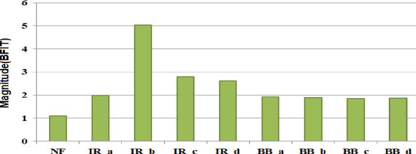
Bearing Health Condition

Fig.11. Representation of BFIT at various health conditions of bearing

The mean±σ analysis and box plot analysis of TDFs of vibration database have revealed that peak, RMS, kurtosis, and skewness features have shown reliable results among all considered TDFs to discriminate the health conditions of bearing. The results of BFIT analysis of TDFs have also shown that it is very effective to identify bearing defects in its early stage.

• IV.    Conclusion

In this paper, the time-domain features of vibration signals have been used to diagnose bearing defects. The single point inner raceway and ball defect severities of rolling-element ball bearing have been studied under operating loads 0Hp, 1HP, 2HP, and 3HP. The results have revealed that TDFs of vibration signals are almost independent of operating loads. The results of the mean±σ analysis have depicted that peak, RMS, kurtosis, and skewness features are comparatively more reliable to identify the bearing defects. The results of the box plot analysis have shown that it is an effective and appropriate statistical approach to envisage the small variations in TDFs. The results of the proposed third method have demonstrated that BFIT values for NF bearing are less than 1.1, while greater than 1.8 for faulty bearing. From BFIT analysis, it also has been observed that initially its value increases with IR fault severities then decreases, but always greater than NF bearing. It signifies that the proposed method is more appropriate and efficient to identify incipient IR faults compared to other considered statistical methods. However, time-domain analysis of vibration signal has the shortcomings of low sensitivity and accuracy of fault prediction. Therefore, these features can be incorporated with soft computing method for better fault prediction accuracy.