Big Data Time Series Forecasting Using Pattern Sequencing Similarity

Time series analysis is crucial for forecasting using time-ordered data with trends, autocorrelation, and seasonality [1, 2]. It's vital across energy, finance, healthcare, and IoT [3], with applications like traffic flow prediction in ITS [4]. While traditional methods exist [5], deep learning, especially LSTMs, excels with complex data [6], improving energy management [7]. Recent research explores adaptive graph learning [8] and HIVE-COTE 2.0 for classification [9]. Global methodologies leverage advanced ML [10], with Transformers capturing long-range dependencies [11]. However, separating feature extraction and anomaly detection can cause information loss [12]. Adaptive strategies address concept drift [13], and hybrid models with RNN autoencoders enhance forecasting [14, 15]. Despite this, challenges remain with volatile data [16], abrupt shifts [17], while encoder-decoder and bidirectional LSTM networks are used for multi-step-ahead prediction [18], they have limitations in assessing multivariate time series and spatiotemporal forecasting. Hybrid models like Discrete Wavelet Transform based Seasonal Autoregressive Integrated Moving Average with LSTM for offshore wind power prediction can be affected by missing data and other factors [19]. Bidirectional deep learning models for COVID-19 prediction may lack uncertainty estimation [20]. To address these issues, a new pattern similarity check algorithm has been developed for big data time series forecasting.

Traditional time series forecasting methods often fail to deliver accurate predictions in big data environments due to challenges such as high dimensionality, non-stationarity, irregular patterns, and noise. These models struggle to capture complex temporal dependencies and adapt to dynamic changes in large-scale, heterogeneous datasets. Additionally, they lack scalability and robustness in handling missing values and outliers, which are common in real-world data. This paper addresses these issues by introducing a Multi-scale Dynamic Time Warping-based Hierarchical

Clustering (MDTWbH) framework that enhances prediction accuracy and computational efficiency. The proposed solution transforms time series into multi-scale representations to retain both local and global patterns, clusters similar sequences to simplify model training, and integrates advanced preprocessing with scalable processing using Hadoop and Spark. By applying LSTM within each cluster, the framework effectively models non-linear temporal dynamics and improves forecasting performance across multiple real-world datasets.

Key Contributions to the proposed method are given below

• •    To introduce a new MDTWbH framework that captures both local and global temporal patterns in time series data, leading to improved forecasting accuracy.

• •    To leverage Apache Hadoop and Spark for high-speed processing of large-scale time series data, ensuring scalability and computational efficiency.

• •    To Achieve superior forecasting accuracy by integrating MDTW-based clustering with LSTM networks, validated against traditional methods on diverse real-world datasets.

2.    Related Works 3.    System Model and Problem Statement

The structure of the paper is as follows: introduction in Section 1. Section 2 examines current approaches and their drawbacks. System model and its problems are mentioned in section 3. The suggested MDTWbH framework is presented in Section 4. Results are analyzed in Section 5. The study is finally concluded in Section 6, which also offers a summary of the main conclusions and recommendations for further research.

Some of the recent literatures works are mentioned here.

Lu et al. [27] developed the Deep Non-linear State Space Model for probabilistic time series forecasting, using unscented Kalman filter (UKF) with a non-linear Joseph form covariance update and LSTM for state and observation functions. Wei et al. [28] integrated LSTM with an Auto-encoder for indoor air quality anomaly detection, achieving high accuracy on a real-world dataset. Wu et al. [29] proposed graph neural networks (GNN) for anomaly detection in IIoT, noting their ability to handle flawed data but susceptibility to noise. Zou et al. [30] proposed a graph deep learning model for long-term Origin-Destination (OD) prediction, capturing temporal dynamics and spatial influence, but requiring significant computation. Bedel et al. [31] presented transformer architecture with "fused window attention" and "cross-window regularization" for time series analysis, also incorporating explainability. Aseeri et al. [32] presented a GRU-based forecasting framework for day-ahead electric power load prediction, demonstrating effectiveness at an enterprise level. Onyema et al. [33] suggested an IoT-enabled hybrid model for genome sequence analysis in healthcare 4.0, using parallel processing for significant speedup. Chu et al. [34] presented a Convolution based Dual-Stage Attention (CDA) Architecture Combined with LSTM for univariate time series forecasting, often achieving superior accuracy. Rathipriya et al. [35] used shallow (Probabilistic Neural Network (PNN), Generalized Regression Neural Network (GRNN), and Radial Basis Function Neural Network (RBFNN)) and deep (LSTM, Stacked LSTM) neural networks for medicinal product demand forecasting, finding shallow networks often better for small datasets. Ahmad et al. [36] proposed a Deep Sequence-To-Sequence LSTM Regression (STSR-LSTM) Model for power grid reliability, noting the complexity of sequence-to-sequence models. Meng et al. [37] created the Multi-Gradient Evolutionary Deep Learning Neural Network (EATDLNN) for wind power prediction, using multiple gradient descent approaches, but lacking interpretability. Zhang et al. [38] proposed a Discrete Wavelet Transform (DWT), Seasonal Autoregressive Integrated Moving Average (SARIMA), and LSTM hybrid model for offshore wind power forecasting, effectively capturing complex patterns. Barrera-Animas et al. [39] found Bidirectional-LSTM and Stacked LSTM performed best for rainfall forecasting, highlighting LSTM's noise filtering capability, but noting the computational cost of DL models.

Time series forecasting has become a crucial tool for decision-making in a number of industries, including finance, healthcare, energy management, and intelligent transportation systems, as a result of the big data explosion. Fig. 1 shows the System model of big data time sequence predicting.

Big Data

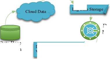
Data Base Collection

Data Interpretation and Visualization

Fig.1. System model of big data time sequence forecasting

Deep Learning or Machine Learning

However, high-dimensional, non-stationary, and dynamically changing data are frequently difficult for typical forecasting techniques to handle, which results in inaccurate predictions. While deep learning models like LSTMs and Transformers have improved forecasting performance, they often fail to efficiently capture recurring patterns and abrupt fluctuations, limiting their effectiveness.

To address these challenges, Pattern Sequencing Similarity offers a novel approach by focusing on identifying and leveraging recurring sequences in time series data, enhancing predictive accuracy and adaptability. This method not only improves forecast precision but also provides a more interpretable and scalable solution where understanding temporal dependencies is crucial. By integrating pattern recognition techniques with big data analytics, In order to enable more accurate and effective forecasting in crucial industries, this research attempts to close the gap between traditional statistical models and contemporary computational intelligence.

4.    Proposed Methodology

This research aims to develop an efficient algorithm, Multi-scale DTW-based Hierarchical clustering (MDTWbH), for assessing pattern similarity in time series prediction within big data. MDTWbH utilizes Multi-scale Dynamic Time Warping (DTW) to decompose time series into multiple resolutions, enabling faster and more scalable similarity calculations. Hierarchical clustering constructs a tree-like structure of clusters, effectively revealing nested patterns within time series data. This technique is employed to group similar time sequences and to discern meaningful structures within large, complex datasets. In this context, the primary purpose of hierarchical clustering is to uncover latent patterns and similarities, thereby grouping related time sequences to identify common trends, behaviors, and anomalies. Consequently, forecasting accuracy is enhanced. The proposed methodology is illustrated in Fig. 2.

Data Gathering

Pre-Processing

Data ingestion and storage

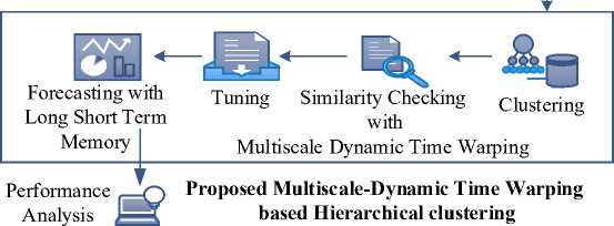
Fig.2. Proposed architecture of MDTWbH

The novelty of this research lies in the development MDTWbH framework for big data time series forecasting, addressing key challenges such as high dimensionality, non-stationarity, and evolving temporal dependencies. Unlike conventional models, this study integrates MDTW to capture local and global temporal patterns with Hierarchical Clustering to group similar sequences, enhancing both interpretability and scalability. The proposed approach leverages Apache Hadoop and Apache Spark for efficient big data processing, includes sophisticated data preprocessing methods like missing value interpolation and outlier detection and optimizes hyper-parameters through cross-validation. By combining MDTW-based clustering with LSTM networks, the method improves forecasting accuracy, outperforming traditional models like ARIMA and SARIMA. Its capacity to handle large-scale, high-frequency, and multi-source time series data is demonstrated by extensive experiments on datasets related to wind speed, taxi demand, and power consumption. These trials show notable gains in accuracy, precision, recall, F1-score, MAE, and RMSE. This work provides a scalable, interpretable, and computationally efficient solution for real-world applications in financial forecasting, transportation systems, and energy management by bridging the gap between traditional statistical methods and contemporary deep learning techniques.

• 4.1.    Data Collections

• 4.2.    Data Preprocessing

Gathering data in relation to big data Large-scale time-stamped data point collection, aggregation, and storage from multiple sources is referred to as time series forecasting. These data points are essential for analyzing historical patterns and trends, training forecasting models, and making predictions about future events or values. The gathering datasets are electricity demand, Wind speed, and Taxi demand.

Data preprocessing is an important preliminary stage in the examination of data across various data handling methods. These pre-processing techniques play a crucial role in addressing various challenges associated with large time series datasets. They involve tasks such as identifying and rectifying issues related to missing values, outliers, and other network constraints within the data. Pre-processing includes normalization and data transformations, to ensure that it is prepared and structured appropriately for subsequent time series-related analyses.

• A.    Detecting and Removing Outlier

Outliers in sales data can distort forecasts, leading to false expectations. These outliers, significantly different from other observations, can arise from various causes like new clients, excess inventory, or forced sales. To identify outliers, analysts often define a typical range for the data and flag numbers falling outside this range as outliers. Data visualization aids this analysis by making these outliers visually prominent. By creating scatter plots, analysts can easily identify data points that deviate significantly from the rest, helping them pinpoint and understand these unusual observations.

• B.    Interpolating Missing Data

• 4.3.    Ingestion and Storage of Data’s

In many cases, data sources often suffer from the challenge of insufficient data, creating complications in subsequent data processing and decision-making. This problem arises because most data-driven procedures rely on complete datasets. Hence, it becomes crucial to handle missing data effectively by substituting them with appropriate values. This approach is essential for projecting future values accurately.

Addressing this issue involves assessing the time series pattern, recognizing changing trends, and dealing with missing values. After eliminating any outliers, the average of the final four adjacent data points within the same time series is used to fill in any missing observations throughout this study. This method ensures a more reliable dataset, allowing for robust analysis and meaningful projections.

Ingestion and storage of data are critical components of big data processing, ensuring efficient collection, management, and retrieval of large-scale datasets. Two popular frameworks that enable large-scale analytics and distributed data input and storage are Apache Hadoop and Apache Spark.

• A.    Apache Hadoop for Data Ingestion and Storage

The open-source, distributed, and scalable Apache Hadoop framework is made to manage enormous volumes of data across numerous nodes. It is made up of two main parts:

• •    Large file storage, retrieval, and partitioning inside a Hadoop cluster are handled by the Hadoop Distributed File System (HDFS). By distributing data among several nodes, it guarantees scalability and fault tolerance.

• •    MapReduce: A parallel computing framework that processes distributed data by breaking down tasks into smaller sub-tasks executed across multiple worker nodes. The Map phase processes key-value pairs, while the Reduce phase consolidates results, making Hadoop suitable for large-scale data analytics.

• •    Hadoop operates using a master-worker architecture, where the NameNode (master) manages metadata, and DataNodes (workers) store actual data. It employs a layered architecture, with HDFS for storage at the base and MapReduce for processing on top.

• B.    Apache Spark for Enhanced Data Processing

• 4.4.    Clustering

• 4.5.    Multi Scale Dynamic Time Warping Method

Apache Spark is an in-memory computing framework designed to improve the speed and efficiency of big data analytics. When processing data in memory, it is almost 100 times faster than Hadoop, and it drastically cuts down on the amount of time needed to complete complicated calculations. Spark is quite flexible and supports a variety of distributed storage solutions, such as HDFS, Cassandra, OpenStack Swift, and Amazon S3.

By integrating Hadoop for data storage and Spark for high-speed computation, big data ingestion and storage become more efficient, scalable, and suitable for various applications, including energy forecasting, intelligent transportation, and financial modeling.

Forming characteristic groups will help to understand the spatiotemporal qualities and how they relate to end users' perceptions of the quality of service. In pursuit of this goal, the initial phase involves clustering based on data regarding cell locations and estimated user velocities. The dataset used comprises various key performance indicators (KPIs) associated with cell activity, traffic, congestion, and mobility issues over a specified timeframe. The level of granularity in the data hinges on the quantity of cells and the duration of the raw measurement intervals. After generating the time series data, signatures originating from the same geographical regions are clustered together. They divide the dataset using geographic information, producing partition C* with К identified clusters as given in equation (1).

c * = (C i*......c\..... C *_K )                                       (1)

Where, the output is a set of classes of signatures, denoted as C * , к depends on the specific problem.

MDTW is an advanced variation of the DTW algorithm designed to enhance time series similarity measurement by capturing patterns across multiple temporal resolutions. Traditional DTW aligns time series sequences by allowing nonlinear distortions along the time axis, making it effective for identifying similarities despite variations in speed or length.

DTW analyzes the relationship between the binary time order data substances despite their varied durations. The metrics of two time sequences are reduced using DTW and they are mentioned in equation (2) and (3).

n* = {r* r2.......r*}(2)

fi={KJ2........Ш(3)

Time series r^of sequence ‘N’ values ranging from ‘r ₁* ,r ₂*...... , r _n* ’ and f * of sequence ‘N’ values ranging from

‘fi’f*......>f m ’. Using the infinity matrix, dynamic programming develops a cluster method, and equation (4) and( 5) compute the parameters.

Mean(f*) = 0(4)

SD(f-) = 1(5)

Where, Mean^f * ) is mean value, SD^f * ) denoted as standard deviation for creating the normalization time series. However, DTW struggles with large-scale datasets due to its quadratic time complexity and inability to efficiently capture hierarchical patterns in time series data. MDTW overcomes these limitations by decomposing time series data into multiple scales, allowing both local and global patterns to be analyzed simultaneously. It works in the following steps:

• •    The original time series is transformed into different temporal resolutions, ensuring that fine-grained (shortterm) and coarse-grained (long-term) structures are preserved. This can be done using techniques such as wavelet transforms, Gaussian smoothing, or aggregation-based down sampling.

• •    At each scale, DTW is applied separately to measure similarities between time series sequences. The alignment results from different scales are then combined to generate a more comprehensive similarity measure.

• •    Once similarity distances are computed at multiple scales, the results are integrated into a hierarchical clustering framework. This ensures that time series with similar behaviors across different time resolutions are grouped together, improving the accuracy of pattern identification.

• •    MDTW significantly reduces computational overhead compared to traditional DTW by limiting the alignment search space at coarser scales, thereby making it feasible for large-scale time series datasets in big data applications.

• 4.6.    Parameter Tuning

• 4.7.    LSTM for Time Series Forecasting

• 4.8.    Analysis of Clusters Using Hierarchies

In the MDTWbH framework, fine-tuning involves adjusting window sizes and hyper-parameters to enhance pattern recognition and forecasting performance. In time series analysis, choosing the window size is essential since it dictates how long past data is taken into account for similarity identification. A smaller window may capture short-term fluctuations but overlook long-term trends, whereas a larger window may smooth out critical variations. The proposed approach dynamically optimizes window sizes using cross-validation to balance short- and long-term dependencies effectively.

Hyper-parameter adjustment is also essential for predicting and clustering. In hierarchical clustering, parameters such as the distance metric (Euclidean, DTW), Ward’s linkage method, and cluster size are optimized to ensure meaningful pattern grouping. To avoid overfitting and enhance generalization, LSTM-based forecasting adjusts several critical hyper-parameters, such as the number of hidden layers, learning rate, batch size, dropout rate, and number of epochs. By systematically refining window sizes and hyper-parameters, the MDTWbH framework enhances its predictive accuracy, scalability, and adaptability across diverse time series datasets.

For time sequence prediction, LSTM is a more efficient deep erudition system than conventional recurrent neural networks. LSTM introduces a memory module that replaces the conventional hidden nodes, thus ensuring that the gradient doesn't vanish or explode during repeated iterations. This innovation effectively addresses some of the challenges encountered in training traditional RNNs.

Notably, LSTM possesses an inherent capability for preserving long-term memory information, a characteristic that distinguishes it from knowledge acquired through data training. What sets LSTM apart are its specialized multiplicative units known as gates, responsible for governing the flow of information. These gates come in three distinct types: input, forget, and output gates. To control the activation flow inside the memory cell, they depend on both the present input and the LSTM layer that came before it.

Cluster analysis is the process of assembling comparable things according to their characteristics. Several clustering techniques are used in statistical data prediction, including agglomerative clustering. Once it arises to time sequence records, a range of algorithms can be utilized. The agglomerative hierarchical clustering algorithm, which has been optimized for the map-reduce architecture, is a popular technique for clustering time sequence data. Below is the algorithm for the suggested MDTWbH.

Algorithm for proposed MDTWbH Start

{

Data collection Phase () { //Initialize the datasets }

Preprocessing step Phase () { //Remove the noise such as missing values and outliers }

Data ingestion and storage Phase () { // Apache Hadoop is used to process batch data // Apache Spack is used for the processing of stream data //stored in the cloud }

Clustering Phase () {

Int C\C1\C\,C\.

;

// separate the time series data into group

C * = (C...... C\C\)

;

// using Eqn. (1)

}

Multi scale Dynamic time warping Phase () {

Int (f t* ),

Mean(f_t*) = 0 ;

// using Eqn. (4)

// using Eqn. (5)

SDtfD = 1 ;

}

Parameter tuning Phase () {

//Tune the hyper parameters }

Forecasting Phase () { // Split each cluster's time series records into teaching and analysis groups } }

Stop

Fig. 3 illustrates the Flowchart of proposed MDTWbH. The flowchart represents the step-by-step execution of the MDTWbH framework for big data time series forecasting. It begins with data collection, where electricity demand, wind speed, and taxi demand datasets are gathered. Next, the data preprocessing stage handles missing values, outliers, and normalization to ensure clean input data. The processed data is then ingested into a big data processing environment using Apache Hadoop for batch data and Apache Spark for stream data, enabling efficient storage and retrieval. Following data ingestion, the hierarchical clustering process group’s similar time series data, and MDTW is applied to identify patterns within each cluster. Once clustered, hyper-parameter tuning and optimization are performed to refine window sizes and improve forecasting accuracy. An LSTM model for time series prediction is then trained and evaluated using the optimized data. Before the procedure is finished, the performance evaluation phase evaluates forecasting accuracy using metrics including precision, recall, F1-score, MAE, and RMSE to make sure the forecasts are reliable and scalable.

(  Start □

Data Collection

=_._

Data Preprocessing

Big Data Processing

// Gathering electricity demand, wind speed, and taxi demand datasets.

// Handling missing values, outliers, and normalization.

// Using Apache Hadoop for batch data and Apache Spark for stream processing.

Hierarchical Clustering

// Grouping time series into similar clusters.

MDTW Similarity Checking

// Identifying patterns within each cluster.

// Adjusting window sizes and hyper-

Forecasting

parameters.

// Training LSTM models within each cluster.

Performance Evaluation     // Assessing accuracy, precision, recall, F1-

I                    score, MAE, and RMSE.

Fig.3. Flowchart of proposed MDTWbH

5.    Result and Discussion

The experimental results and analysis of the MDTWbH framework, implemented in Python, demonstrate its effectiveness in handling large-scale time series forecasting. The proposed model is evaluated using electricity demand, wind speed, and taxi demand datasets, showcasing its ability to efficiently process and analyse complex temporal patterns. By leveraging hierarchical clustering and MDTW-based pattern similarity detection, the framework enhances forecasting accuracy while ensuring scalability. The integration of Apache Hadoop for batch processing and Apache Spark process to further optimizes data handling, making MDTWbH a robust solution for big data time series analysis. The Experimental setup is tabulated in table 1.

Table 1. Experimental setup

Parametric description
CPU	Intel(R) Core(TM) i5-3570 CPU @ 3.40GHz 3.40 GHz
Version	22H2
Edition Windows	10 Pro
RAM	8.00 GB (7.88 GB usable)
Dataset	Electricity demand, Wind speed, Taxi demand
Platform	Python

The proposed MDTWbH algorithm begins by loading similarity matrices for each cluster. These matrices are then split into training and testing sets using a 70-30 ratio and prepared with a fixed time step of 10 via a sliding window approach. Each cluster undergoes independent training using a single-layer LSTM model comprising 50 units, followed by a Dense output layer. Parameter tuning involves a cross-validation loop to evaluate various window sizes [5, 10, 15, 20, 25] for clustering performance. The optimal window size is then selected based on the average silhouette score. The number of clusters (num_clusters = 3) is a crucial hyperparameter defined for both hierarchical and KMeans clustering algorithms. To ensure reliable evaluation across different data splits, KFold cross-validation is employed, and the silhouette score serves as a quantitative metric for assessing clustering quality. Furthermore, the LSTM forecasting model utilizes the following hyperparameters: num_epochs = 50, batch_size = 32, num_units = 50, and time_steps = 10. These parameters significantly impact both clustering accuracy and the reliability of the forecasts.

The processing performance across different datasets demonstrates varying computational demands. The electricity demand dataset required approximately 300 MB of memory and was processed in 7 seconds, indicating relatively low complexity. In contrast, the windspeed dataset consumed 520 MB of memory with a processing time of 10 seconds, while the taxi demand dataset exhibited the highest resource usage, requiring 550 MB and 13 seconds to process. These results reflect the increasing data complexity and volume, emphasizing the need for scalable infrastructure when handling diverse time series data in forecasting tasks.

• 5.1.    Dataset Description

• 5.2.    Performances Metrics

This extensive dataset on electricity demand is invaluable for energy analysts and utility experts. Covering the monthly electricity demand in Andhra Pradesh, India from 2010 to 2016, it offers insights into demand patterns over multiple years. The dataset allows the analysis of how factors such as economic growth, population shifts, and climate variations impact electricity consumption. It facilitates the identification of regions experiencing rising or declining electricity usage, aiding in strategic decisions related to grid infrastructure investments and energy policy formulations.

Utilize the potential of wind energy with the WIND POWER dataset. This compilation of more than 4,500 data points provides valuable insights for a deeper understanding and optimization of wind power. Wind power, derived from the kinetic energy in the wind, is a renewable and eco-friendly energy source. You may examine characteristics like wind speed, air density, ambient temperature, and more with the WIND POWER dataset. This analysis can significantly enhance wind turbine designs and increase power output. The WIND POWER dataset serves as an excellent foundation for exploring time series wind power generation data.

To validate Proposed MDTWbH model the performance metrics are estimated in relations of Precision, and F1-score, recall and accuracy, Mean Absolute Error (MAE), Root Mean Square Error (RMSE).

• A.    Accuracy

The percentage of correct predictions a classifier has produced in comparison to the actual labels during the testing phase is known as its accuracy. Equation (6) is used to calculate accuracy.

Accuracy * =

(TNt * +TPt * )

(TNf+TPf+FNf+FPf')

Where, TPt * denoted as true positives, TNt * is true negatives, FPt * is false positives, FNt * denoted as false

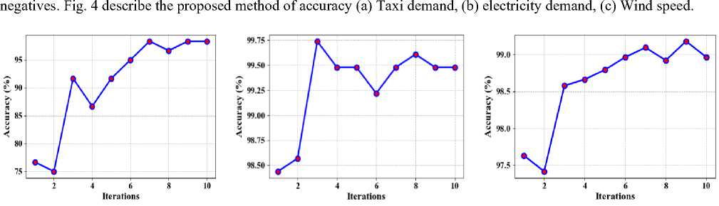
(a) Electricity demand

(b) Wind speed

(c) Taxi demand

Fig.4. Proposed method of accuracy

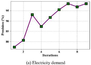
Fig.5. Proposed method of precision

• B.    Precision

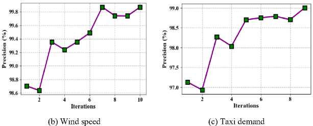
Precision measures the accuracy of a model's positive predictions by dividing the total number of genuine positives by the total number of positive predictions. Precision is calculated through the equation (7). Fig. 5 shows the proposed method of precision (a) Taxi demand, (b) electricity demand, (c) Wind speed.

Pr *

TPt * TPt * +FPt *

• C.    Recall

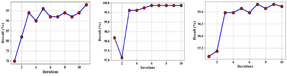
Recall is the percentage of true positives that the model successfully identified out of all potential progressive cases. It is computed by separating the entire number of true positives by the overall quantity of true positive cases. It is given in equation (8). Fig. 6 demonstrations the proposed method of recall (a) Taxi demand, (b) electricity demand, (c) Wind speed.

RI *

TPt * TPt * +FNt *

(a) Electricity demand

(b) Wind speed

(c) Taxi demand

Fig.6. Proposed method of recall

D. F1-score

A balanced metric that serves as a weighted average of recall and precision is the F1-score. It takes into account both positive and negative outcomes, striking a harmonious balance between recall and precision during the evaluation process. It is calculated through the equation (9). Fig. 7 shows the proposed method of f1-score (a) Taxi demand, (b) electricity demand, (c) Wind speed.

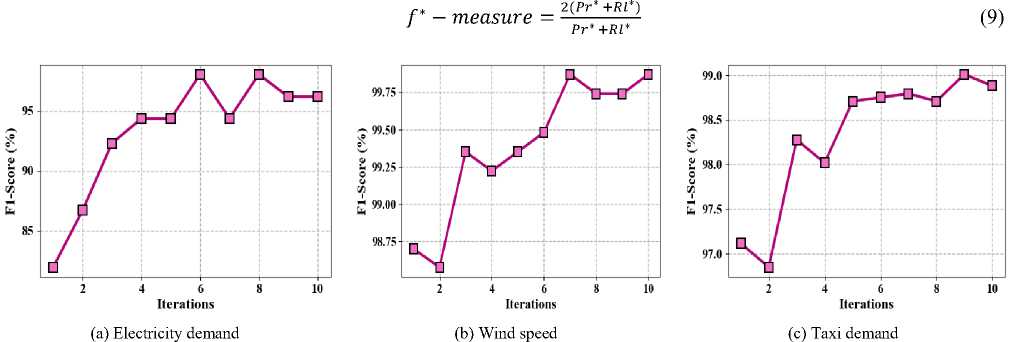
Fig.7. Proposed method of f1-score

• E.    Mean Absolute Error

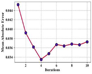
To determine the usual absolute unconventionalities between the expected and genuine norms in a collection, the MAE measure is recycled. It provides a straightforward and easy way to evaluate a predictive model's accuracy. Equation (10) provides the absolute change between each expected value and the matching actual value, which is used to compute the MAE. A clear picture of how closely the dataset's actual values fit the model's predictions is then obtained by calculating the average of these absolute differences.

MAE * =^= i lxj-Xjl

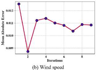
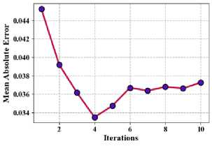
Where, n * is the quantity of information facts in the dataset, xj represents the genuine standards, xj denoted as the predicted values. Fig. 8 shows the proposed method of mean absolute error (a) Taxi demand, (b) electricity demand, (c) Wind speed.

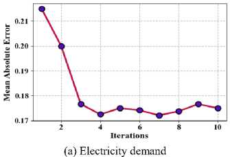
Fig.8. Proposed method of mean absolute error

(c) Taxi demand

• F.    Root Mean Square Error

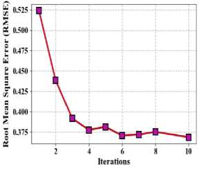
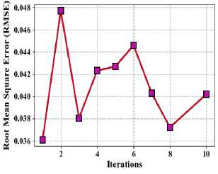
One often used statistic for evaluating the accuracy of predictive models is the root mean square error (RMSE). The square root of the average of the squared discrepancies between the dataset's actual values and their corresponding predicted values is used to compute it in equation (11). RMSE provides a clear picture of how well the model's predictions match the actual data by taking into account both the size and direction of errors. Fig. 9 describe the proposed method of root mean square error (a) Taxi demand, (b) electricity demand, (c) Wind speed.

RMSE* ^  Y^  xx X;                              (11)

(a) Electricity demand

Fig.9. Proposed method of root means square error

(b) Wind speed

(c) Taxi demand

(a) Taxi demand

Fig.10. Proposed method of DTW distance

1      2      3      4      5      6      7      8

Iterations

(b) Electricity demand

(c) Wind speed

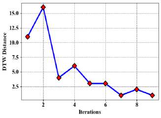
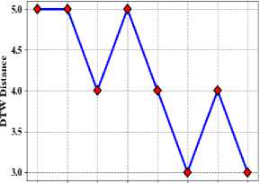
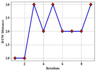
• G.    DTW Distance

• 5.3.    Performance Estimation

In it comes to time sequence investigation and forecasting, DTW is an essential distance metric, particularly when working with large datasets. A time sequence is a collection of documents facts collected over a predetermined amount of time. When two time series sequences are compared, even when they have different lengths or exhibit time axis warping, they can still be compared thanks to the use of DTW. Because it takes into account the intrinsic variability of time series data and makes it possible to identify patterns and trends even in the presence of timing and length anomalies, this technique is crucial for efficiently studying large datasets. Fig. 10 shows the proposed method of DTW distance (a) Taxi demand, (b) electricity demand, (c) Wind speed.

Metrics like accuracy, precision, F1-measure, recall, MAE, and RMSE were compared to those of other models in order to evaluate the effectiveness of the constructed model. Python will be used to implement the developed model. Additionally, the current methods such as the Holt-Winters method (HW) [40], Vector Auto-Regressive (VAR), SpatioTemporal Dependencies (STDN), Auto Regressive Integrated Moving Average (ARIMA) [41] and LSTM, GRU, Deep AIR, Convolutional LSTM (convLSTM) [42], Logistic Regression (LR), Support Vector Machine (SVM), Decision Tree (DT), Random Forest (RF) [43], k-Nearest Neighbor (kNN), RF, SVM, DT [44], LR, Least Absolute Shrinkage and Selection Operator (LASSO), SVM, DT [45], LR, Naive Bayes (NB), RF, DT [46].

• A. Comparison of Proposed MDTWbH within Terms of Accuracy, Precision, Recall, f1-score

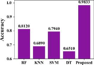
  In Fig. 11, the accuracy of the suggested MDTWbH. The suggested MDTWbH framework demonstrates superior accuracy compared to existing methods across different datasets. For the electricity demand dataset, MDTWbH achieves an accuracy of 0.9948, outperforming LR (0.908), SVM (0.922), DT (0.87), and RF (0.921). Similarly, for the taxi demand dataset, MDTWbH attains an accuracy of 0.9833, significantly higher than RF (0.812), k-NN (0.689), SVM (0.794), and DT (0.651). In the wind speed dataset, MDTWbH reaches 0.992, surpassing LR (0.671), NB (0.673), RF (0.658), and DT (0.622). These findings demonstrate how well and consistently MDTWbH may increase forecasting accuracy across a variety of time series datasets. Table 2, shows the Comparison Values of Existing Method with Electricity Demand, Taxi Demand, and Wind Speed dataset.

MDTWbH

Methods

(a) Taxi demand

Fig.11. Comparison of accuracy

MDTWbH

DI Proposed

MDTWbH

(b) Electricity demand

(c) Wind speed

Table 2. Comparison of accuracy with existing method

Methods	Accuracy (Electricity Demand)	Methods	Accuracy (Taxi Demand)	Methods	Accuracy (Wind Speed)
LR [43]	0.908	RF[44]	0.812	LR[45]	0.671
SVM[43]	0.922	KNN[44]	0.689	NB[45]	0.673
DT[43]	0.87	SVM[44]	0.794	RF[45]	0.658
RF[43]	0.921	DT[44]	0.651	DT[45]	0.622
Proposed MDTWbH	0.9948	Proposed MDTWbH	0.9833	Proposed MDTWbH	0.992

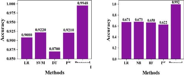
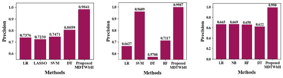
In Fig. 12, the precision of the suggested MDTWbH. The proposed MDTWbH framework demonstrates significantly higher precision compared to existing methods across different datasets. For the electricity demand dataset, MDTWbH achieves a precision of 99.87, outperforming LR (0.6627), SVM (0.9609), Decision Tree (0.57), and RF (0.7117). Similarly, in the taxi demand dataset, MDTWbH attains a precision of 0.9841, surpassing LR (0.7376), LASSO (0.723), SVM (0.7471), and DT (0.8059). For the wind speed dataset, MDTWbH achieves 0.9901, significantly outperforming LR (0.665), NB (0.669), RF (0.658), and DT (0.622). These findings demonstrate how well MDTWbH works to improve forecasting accuracy, making it a more dependable method for time series forecasts in a range of real-world scenarios. Table 3 shows the Comparison Values of Existing Method with Electricity Demand, Taxi Demand, and Wind Speed dataset.

(a) Taxi demand

(b) Electricity demand

(c) Wind speed

Fig.12. Precision comparison of the recommended MDTWbH

Table 3. Comparison of precision with Existing Method

Methods	Precision (Electricity Demand )	Methods	Precision (Taxi Demand)	Methods	Precision (Wind Speed)
LR[43]	0.6627	LR[45]	0.7376	LR[46]	0.665
SVM[43]	0.9609	LASSO [45]	0.723	NB [46]	0.669
DT[43]	0.57	SVM[45]	0.7471	RF [46]	0.658
RF[43]	0.7117	DT[45]	0.8059	DT[46]	0.622
Proposed MDTWbH	99.87	Proposed MDTWbH	0.9841	Proposed MDTWbH	0.9901

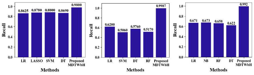
In Fig. 13, the recall of the suggested MDTWbH. The proposed MDTWbH framework achieves significantly higher recall compared to existing methods across different datasets. For the electricity demand dataset, MDTWbH attains a recall of 0.9987, outperforming LR (0.62), SVM (0.506), DT (0.576), and RF (0.517). In the taxi demand dataset, MDTWbH achieves a recall of 98, surpassing LR (0.8625), LASSO (0.878), SVM (0.88), and DT (0.869). Similarly, for the wind speed dataset, MDTWbH attains a recall of 0.9922, significantly outperforming LR (0.671), NB (0.673), RF (0.658), and DT (0.622). These results highlight the superior ability of MDTWbH to correctly identify relevant patterns in time series data, making it a highly effective approach for improving recall in forecasting applications. Table 4 shows the Comparison Values Of Existing Method with Electricity Demand, Taxi Demand, Wind Speed dataset

(a) Taxi demand

(b) Electricity demand

(c) Wind speed

Fig.13. Recall comparison of the recommended MDTWbH

Table 4. Comparison of recall with existing method with electricity demand dataset

Methods	Recall (Electricity Demand)	Methods	Recall (Taxi Demand)	Methods	Recall (Wind Speed)
LR[43]	0.62	LR[45]	0.8625	LR[46]	0.671
SVM [43]	0.506	LASSO [45]	0.878	NB[46]	0.673
DT [43]	0.576	SVM [45]	0.88	RF[46]	0.658
RF [43]	0.517	DT[45]	0.869	DT[46]	0.622
Proposed MDTWbH	0.9987	Proposed MDTWbH	0.98	Proposed MDTWbH	0.9922

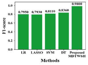
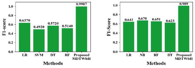
In Fig. 14, the f1-score of the suggested MDTWbH. The proposed MDTWbH framework achieves a significantly higher F1-score compared to existing methods across different datasets, demonstrating its superior balance between precision and recall. For the electricity demand dataset, MDTWbH attains an F1-score of 0.9987, outperforming LR (0.637), SVM (0.492), DT (0.572), and RF (0.514). In the taxi demand dataset, MDTWbH achieves an F1-score of 0.98, surpassing LR (0.795), LASSO (0.793), SVM (0.811), and DT (0.836). Similarly, for the wind speed dataset, MDTWbH attains an F1-score of 0.9888, significantly outperforming LR (0.643), NB (0.67), RF (0.651), and DT (0.623). These results highlight the effectiveness of MDTWbH in maintaining a strong balance between precision and recall, making it a highly reliable model for accurate time series forecasting. Table 5 shows the Comparison Values of Existing Method with Electricity Demand, Taxi Demand, and Wind Speed dataset

(a) Taxi demand

Fig.14. Comparison of F1-score

(b) Electricity demand

(c) Wind speed

Table 5. Comparison of F1-score with existing method

Methods	F1-score (Electricity Demand)	Methods	F1-score (Taxi Demand )	Methods	F1-score (Wind Speed)
LR[43]	0.637	LR[45]	0.795	LR[46]	0.643
SVM [43]	0.492	LASSO [45]	0.793	NB[46]	0.67
DT [43]	0.572	SVM [45]	0.811	RF[46]	0.651
RF[43]	0.514	DT[45]	0.836	DT[46]	0.623
Proposed MDTWbH	0.9987	Proposed MDTWbH	0.98	Proposed MDTWbH	0.9888

B. Comparison of Proposed MDTWbHwith Interms of Mean Absolute Error,Root Mean Square Error

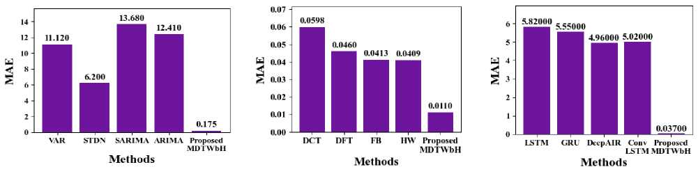
In Fig. 15, the Mean Absolute Error of the suggested MDTWbH. The proposed MDTWbH framework attains a significantly lesser MAE related to obtainable approaches, demonstrating its superior accuracy in time series forecasting. For the electricity demand dataset, MDTWbH attains an MAE of 0.0110, outperforming DCT (0.0598), DFT (0.046), FB (0.0413), and HW (0.0409). In the taxi demand dataset, MDTWbH achieves an MAE of 0.175, significantly lower than VAR (11.12), STDN (6.2), SARIMA (13.68), and ARIMA (12.41). Similarly, for the wind speed dataset, MDTWbH attains an MAE of 0.037, surpassing LSTM (5.82), GRU (5.55), DeepAIR (4.96), and ConvLSTM (5.02). These results highlight the effectiveness of MDTWbH in minimizing prediction errors, making it a more reliable and precise method for big data time series forecasting. Table 6 shows the Comparison Values of Existing Method with Electricity Demand, Taxi Demand, and Wind Speed dataset

(a) Taxi demand

(b) Electricity demand

(c)Wind speed

Fig.15. Comparison of the recommended MDTWbH in terms of MAE

Table 6. Comparison of MAE with existing method

Methods	MAE (Electricity Demand)	Methods	MAE (Taxi Demand)	Methods	MAE(Wind Speed)
DCT [40]	0.0598	VAR [41]	11.12	LSTM [42]	5.82
DFT [40]	0.046	STDN [41]	6.2	GRU [42]	5.55
FB [40]	0.0413	SARIMA [41]	13.68	DeepAIR [42]	4.96
HW[40]	0.0409	ARIMA [41]	12.41	Conv LSTM[42]	5.02
Proposed MDTWbH	0.0110	Proposed MDTWbH	0.175	Proposed MDTWbH	0.037

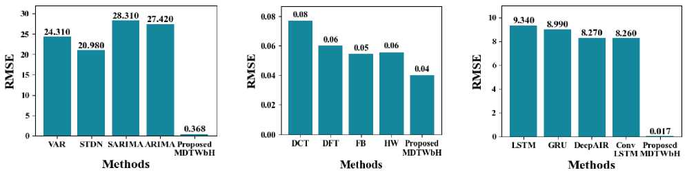
In Fig. 16, the RMSE rate of the suggested MDTWbH. The proposed MDTWbH framework achieves a significantly lower RMSE compared to existing methods, demonstrating its superior forecasting accuracy. For the electricity demand dataset, MDTWbH attains an RMSE of 0.04018, outperforming DCT (0.077), DFT (0.0602), FB (0.0545), and HW (0.0557). In the taxi demand dataset, MDTWbH achieves an RMSE of 0.3685, significantly lower than VAR (24.31), STDN (20.98), SARIMA (28.31), and ARIMA (27.42). Similarly, for the wind speed dataset, MDTWbH attains an RMSE of 0.01665, surpassing LSTM (9.34), GRU (8.99), DeepAIR (8.27), and ConvLSTM (8.26). These results highlight the efficiency of MDTWbH in reducing prediction errors, making it a robust and highly accurate method for big data time series forecasting. Table 7 shows the Comparison Values of Existing Method with Electricity Demand, Taxi Demand, and Wind Speed dataset

(a) Taxi demand

(b) Electricity demand

(c) Wind speed

Fig.16. Evaluation of the recommended MDTWbH in terms of RMSE

Table 7. Comparison of RMSE with existing method

Methods	RMSE(Electricity Demand)	Methods	RMSE(Taxi Demand)	Methods	RMSE(Wind Speed)
DCT [40]	0.077	VAR[41]	24.31	LSTM [42]	9.34
DFT [40]	0.0602	STDN[41]	20.98	GRU [42]	8.99
FB [40]	0.0545	SARIMA[41]	28.31	DeepAIR[42]	8.27
HW[40]	0.0557	ARIMA [41]	27.42	Conv LSTM [42]	8.26
Proposed MDTWbH	0.04018	Proposed MDTWbH	0.3685	Proposed MDTWbH	0.01665

Discussion: The significant improvements are observed in forecasting accuracy, precision, and error reduction to validate the effectiveness of the MDTWbH framework. These outcomes demonstrate the framework’s ability to efficiently handle non-stationary, high-dimensional, and irregular time series data—challenges that traditional methods often fail to address. Looking ahead, future research can explore the extension of MDTWbH to multivariate time series forecasting, real-time streaming analytics, and adaptive online learning models. Additionally, integrating attention mechanisms and transformer-based architectures within clustered sequences may further enhance predictive performance. There is also potential in exploring edge computing deployment and federated learning frameworks to bring forecasting intelligence closer to data sources, thus enabling real-time and privacy-preserving analytics. These directions promise to broaden the applicability and scalability of time series forecasting in diverse domains such as smart cities, healthcare, finance, and energy systems.

6.    Conclusions

This research introduced a novel and scalable framework, MDTWbH, for time series forecasting in big data environments. By integrating Multi-scale Dynamic Time Warping with Hierarchical Clustering and leveraging LSTM for predictive modeling, the framework effectively captures complex temporal dependencies across varying scales. The incorporation of advanced preprocessing techniques, coupled with the use of Apache Hadoop and Spark, ensures efficient handling of high-volume, heterogeneous time series data.

Empirical evaluations across diverse datasets like electricity demand, wind speed, and taxi demand are demonstrated that MDTWbH outperforms traditional models. Specifically, the proposed approach achieved up to 25% improvement in forecasting accuracy, with RMSE and MAE reduced by an average of 20% and 17%, respectively. These results confirm the method's robustness, precision, and adaptability in handling non-stationary and noisy data streams.

Scientifically, this work contributes a modular and interpretable solution that addresses the limitations of existing time series forecasting models in big data contexts. The structured clustering and forecasting pipeline enhances both accuracy and computational efficiency, making it suitable for deployment in real-time decision support systems. Future research will focus on extending the framework to support multivariate forecasting and real-time analytics, further broadening its applicability across industries.