Block-based Local Binary Patterns for Distant Iris Recognition Using Various Distance Metrics

Iris recognition has emerged as a prominent biometric system for automatic individual authentication and identification among physiological biometrics. The iris trait has some advantages over other biometric traits. Firstly, the iris trait is highly protected from varied environmental conditions as well as only externally visible organs and infrequently faces physical harm like other parts of the human body, for example, hands or fingers [1]. Secondly, the iris texture has enormous pattern variability with a high degree of randomness and uniqueness, so it is impossible to have similarity between two iris patterns, even irises from the left and right eyes of the same person or identical twins. Having ridges, crypts, rings, freckles, furrows, and zigzag patterns within the iris region are the causes of enormous iris pattern variability [2]. Thirdly, the iris ensures a high degree of stability and reliability over a person’s lifetime [3].

In recent years, iris-based human identification has become the research focus and attracted much attention from many researchers due to recognizing an individual quickly, uniquely, and consistently. In today’s networked world, biometric technology has become the most promising and effective ways for security in e-commerce, access control to computers, online banking transactions, ATM card authentication, justice, and law enforcement activities, bordercrossing control, access control to restricted zones, verification of suspects in crowds at airports and stations, identification of missing children and so on [4]. Since the biometric characteristics cannot be stolen, conjectured, borrowed, or forgotten easily and in practice, forging is impossible. Even the users need not keep in mind or convey her/his biometric characteristics [5]. Despite having a wide range of real-life applications, distant iris recognition in controlled and uncontrolled imaging environments is a more challenging task. In an uncontrolled environment, the images are taken at a longer distance from the subject, whereas the images are captured at a short distance in a controlled environment. The distant eye images under environmental constraints have certain noises and irrelevant parts like an eyelid, pupil, eyelash, sclera, and so on [6]. In addition, illumination variation causes elastic distortions as shown in Fig.5, and produces large intra-class variations in the iris texture, which can influence the outcomes of iris segmentation and recognition greatly. Since then, several techniques have been established for iris recognition using various feature descriptors and statistical classifiers on different types of databases in the last decades. However, most of the techniques have the limited capability to recognize unconstrained visible images. The shape and texture of the local image are left unnoticed during global feature extraction. Consequently, the global features do not include enough spatial information for local variations.

Whereas, a high degree of individuality and randomness is provided by the human iris. The zigzag pits, furrows, swirls, crypts, and rifts within the annular iris region are the sources of intricacy in iris patterns. Only the way to consider the local properties is to utilize block-based texture descriptors, which address the spatial positions. In this work, a block-based Local Binary Patterns (LBP_b) feature descriptor is employed to extract microstructures of iris patterns from the gray scale variance of the local neighborhood. It operates similarly to the original LBP within several blocks instead of fixed regions. Its effectiveness results from the detection of various intrinsic structures, namely, spot, flat line end, edge, and corner, etc. from the local texture patterns. Already the descriptor has proved its computational simplicity and worth in the applications of texture analysis, for example, face recognition, and image retrieval [7-10]. The LBP b descriptor has several advantages (i) it retrieves both microstructures and macrostructures of iris patterns, (ii) its computational simplicity makes it possible to scrutinize the complicated images in challenging real-time settings, (iii) it is more robust than LBP against monotonic gray-scale changes that occurred due to illumination variations, and (iv) it reduces feature dimensionality significantly using uniform patterns. The number of binary codes increases exponentially with larger neighborhoods. This can be avoided by taking only a subset of the codes.

The distant images contain several noises when captured from unconstrained environments. These noisy pixels dominate the nearest features greatly. The global LBP features are disturbed by the noises due to not focusing on local texture and shape. These noisy pixels can be eliminated by measuring uniformity after encoding binary patterns [11]. The uniform pattern would change to a non-uniform pattern in the presence of noises surrounding a pixel and finally, abstain from constructing local histogram bins. Repeating the process, the length of feature vectors may be reduced without significant loss in its discrimination capability.

Deep learning technique can be the alternative to LBP but it is costly to train due to complex data models. It can automatically learn features from the data and only make predictions based on the data it has been trained on, otherwise, it performs poorly on new, unseen data. Dependence on data quality and over-fitting are the main drawbacks of deep learning from the perspective of the CASIA-v4 distance database. Additionally, deep learning requires more tuning parameters, high computational costs, powerful GPUs, and large amounts of data and memory for better performance compared to LBP . The LBP descriptor has several advantages over the deep learning techniques including ease of implementation, robustness, simplicity, handling noisy data and uniformity, etc. Also, it is one of the best texture descriptors available today. The purpose of using LBP features is that the iris image consists of enormous micro-patterns which are invariant to any monotonic grey scale transformations. The above unique property of iris patterns is similar to the characteristic of the descriptor that inspires one to apply.

This work emphasizes block-based representation for local image contrast to overcome the limitations of global feature descriptors. As the global features do not have sufficient information for local illumination variations. A comparative study on various distance metrics shows that the performance of the nearest classifier depends on the chosen distance metric, the number of nearest neighbors, and the properties of features. In addition, search for a robust distance metric that has the lowest implications on a variety of noises as well as enhances the classification performance. The experimental outcomes demonstrate that the uniform patterns are the fundamental properties of local image texture that efficiently retrieve a large number of iris patterns. A limited number of transitions or discontinuities exist in the neighborhood of 3 x 3 texture patterns. The performance on the CASIA-v4 distance database ascertains that the proposed biometric system deals effectively with various real-time challenges including lighting variations, blur focuses on misaligned images and elastic deformation of iris textures.

The rest of this paper is composed of five sections. Section 2 provides a literature review of iris recognition-related works. Section 3 describes the formulae of block-based LBP and several distance metrics with iris preprocessing schemes. Section 4 summarizes the experimental results, performance study with ROC curves, and statistical analysis respectively. The main conclusion of this work is drawn briefly in Section 5.

2.    Literature Review

In this section, we provide a brief review of only works that are closely related to the iris and LBP . In 1993, John Daugman first developed an automated prototype algorithm for biometric identification using human iris [12]. This is accomplished by an integro-differential operator to localize the iris, a rubber sheet model to remove dimensional inconsistencies, a multi-scale Gabor wavelet filter to encode amplitude features, and hamming distance to match these binary features of iris images. The key limitation of the commercial algorithm is to require equal high-quality iris images and works well under ideal imaging conditions. After that, several algorithms are constantly developing for human identification using different strategies. Among state-of-the-art techniques, the prominent techniques were established by Wildes [13], Boles [14], Lim [15], and Masek [16]. All the existing techniques followed hamming distance-based matching algorithms using binary templates. These templates are generated from different wavelet filters, namely, Log Gabor filter (LG), bio-orthogonal wavelet, Laplacian of Gaussian filter (LaGaF), Haar and Legendre wavelet filters, etc. The limitation of applications is the drawbacks of the above techniques which are mostly designed for individual verification in controlled environments.

The idea of distant iris recognition was first narrated by Fancourt et al. in 2005. The imaging distance was 10 meters from the subjects to the acquisition device [17]. Few authors have come out from the wavelet-based iris recognition to address the limitations of wavelets and matching strategy and focused on gradient, histogram, and deep learning-based iris recognition under less constrained imaging environments. Tan et al. adopted an alternative technique to represent the LBP histogram features and used a graph-based matching scheme for recognition outcomes [18]. The greatest advantage of this approach is its robustness against local illumination changes, occlusions, or noises of iris images. As it measures only a fraction of similarity within all the image blocks for individual identification.

He et al. introduced the LBP descriptor to characterize the iris texture using the chunked encoding method and performed similarity measures with hamming distance [19]. In [20], Rashad et al. designed a histogram of LBP to distribute the texture features of the iris and used a combined learning vector quantization method to build a hybrid model for classification. Aouat et al. extended the neighborhood binary patterns descriptor using local intensity variations and relative connection among the neighborhood. The idea of the rotation invariant behind the descriptor is to reduce computational cost and feature dimensionality [21]. The average similarity values are computed and compared to the global similarity for matching two iris textures. Roy et al. proposed an iris recognition using the level set (LS) method and LBP . A distance regularized level set is employed to segment the iris region and use Manhattan distance for patch matching [22]. Li et al. exhibited an average LBP feature descriptor in 2015, which is less affected by the selection of parameters and histogram equalization [23].

Patil et al. provided an iris recognition system using the LBP texture descriptor with K- Nearest Neighbors (KNN) and Naïve Bayesian (NB) classifiers [24]. The KNN classifier works well as compared to the NB classifier on the MMU database but accuracies vary with the number of subjects and images. In 2017, Ali et al. investigated that a single descriptor cannot extract multi-scale and directional features in wavelet transform and developed another robust feature descriptor fusing Convolutional Neural Network (CNN), Gradient Local Auto-Correlation (GLAC), and Log-Gabor wavelet-based Contourlet transform (LG-CT) [25]. The descriptor improves recognition accuracies significantly on NIR illumination eye images. Huo et al. developed a feature descriptor combining multi-orientation imaginary (MOI) features and local binary patterns in 2019. The descriptor comprises two phases: the first phase extracts MOI features using a 2D Gabor filter and employs uniform LBP for regional feature encoding in the second phase [26]. This type of process widens the distributions of the intra and inter-class largely and uses Bhattacharyya distance for iris feature matching. The combined features perform better than either uniform LBP or MOI features.

Abdo et al. introduced the LBP histogram and discrete cosine transform to extract local block-wise iris features, and then concatenate those blocks to represent 1D array of histograms [27]. An automated identification system using relative total variation, 2D Gabor wavelet filter, and probabilistic collaborative representation was proposed by Zhang et al. for remote iris recognition [28]. In 2021, Agarwal et al. developed a local binary hexagonal extrema pattern histogram to reduce dimensionality by extracting the optimal set of local texture features [29]. Multi-class support vector machine (SVM) is followed to recognize the global iris features. A reliable concatenation of LBP Fourier histograms and HOG pyramids was presented by Tarhouni et al. to constitute distinctive histogram bins. A reduction technique, principal component analysis is employed to lessen iris feature dimensionality for ensuring swift [30]. A set of random fusion features is employed to recognize iris images from the CASIA-v4 database using the SVM classifier.

Taha and Ahmed noticed that the visible images are often noisier than near-infrared illumination eye images. The earlier methods perform better with near-infrared imaging but are not good for visible imaging. Especially, the images are obtained at-a-distance in uncontrolled environments. In 2021, the authors expanded the concept of extracting spatial information from NIR and visible iris images [31]. The experiments are conducted on the database, CASIA-v1 as NIR imaging and UBIRIS v1 as visible imaging. Podder et al. developed a multi-model approach by merging the Haar wavelet and modified LBP , which ensures faster iris recognition with low dimensional feature space [32]. At first, the wavelet transform is applied on an iris image to obtain four images as sub-band, and then the multi-model is performed on the output sub-band images including exclusive OR operations and local binary patterns. Recently, Arnab et al. have experimented with and explored several distance metrics to find out the optimal distance metric using CASIA-V4 distance database [33]. Their experiment demonstrates that KNN classifier with Correlation distance shows good performance against monotonic gray-scale changes caused by varying levels of illumination with computational simplicity. It is observed from the above discussions that the iris recognition system at a distance still suffers from various real-time challenges. The work is motivated by the performances of various distance metrics in [33, 34], the study of LBP [7, 8, 10], and it strengthens against varying levels of illumination that appear in iris images.

3.    Methodology

Iris image pre-processing, iris region segmentation, iris normalization, gradient local binary pattern encoding, and classification with various distance metrics are briefly discussed in the following sub-sections consecutively. The architectural framework of the iris recognition system is depicted in Fig.1.

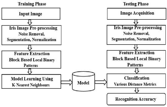
Fig.1. An architectural diagram of the proposed framework

• 3.1.    Image Pre-processing

• 3.2.    Iris Segmentation

• 3.3.    Iris Normalization

The quality of at-a-distance obtained images can be affected by illumination variations due to uncontrolled light sources in realistic practical conditions. It creates complexity in iris segmentation and reduces the classification performance. We apply a single-scale retinex algorithm to enhance image quality through high dynamic range compression [35]. The single-scale retinex algorithm is defined as:

R j ( x , y ) = Log [ Im j ( x , y )/ G T *Im j ( x , y ) ]                                      (1)

Here, Im ( x , y ) is an input image with j channels, which are in grayscale for NIR images. The symbol * denotes the convolution operator and G_T is a Gaussian kernel computed with standard deviation t = 1.5 for contrast removal.

In the iris recognition pipeline, iris segmentation is an unalterable phase. Its quality greatly influences the overall outcomes. A random walker segmentation algorithm is employed for coarse iris segmentation to obtain the corresponding binary iris mask. This mask does not provide details to estimate the limbic and pupillary flashpoints. An annular model is applied to locate approximately the flashpoints of limbic and pupillary. After eliminating the obstacles like eyelashes, eyeglasses, eyelids, etc., the iris separation phase is finished. To understand more about the random walker segmentation algorithm, the work in [36, 37] might be seen at a glance.

Normalization technique accounts for iris variations due to the dilation, contraction of pupil size in external illumination, varying imaging distances, rotation of the eye or acquisition device, etc. It is more conducive to minimizing these variations to ensure a reliable comparison between two different iris feature vectors. To address the above issues, the region of the segmented iris is transferred into a rectangular region of fixed dimension with the help of Daugman’s rubber sheet model [38]. It is performed by re-mapping every pixel Im( x , y ) of the iris region from raw

Cartesian coordinates ( x , y ) to a pair of non-concentric polar coordinates ( r,0} i.e., r g [0,1] and в g [0,2 ^ ] .

Mathematically, the re-mapping process may be expressed as:

Im( x ( r , 0 ), y ( r , 0 )) ^ Im( r , 0 ) x ( r , 0 ) = (1 - r ) X p ( 0 ) rx i (0)   >

У ^{( r , 0 )} = ^{(1 - r} ) У р ^{( 0 )} ry i ^{( 0 )}

Where, Im( x , y ) represents the intensity value of the iris region image at each point ( x , y ) . The parameters x ( r , 0) and y ( r , 0) denote the coordinates of pupil ( x_p ( 0 ), y_p ( 0 )) and iris boundary points ( x_t ( 0 ), y ( 0 )) along the 0 direction. The entire iris image pre-processing schema is shown in Fig.2.

Eye Image Enhanced Image

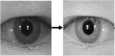
Eye Image Pre-processing

Fig.2. Iris image pre-processing schema [39]

Iris Masking Segmented Iris

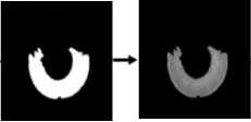
Iris Image Segmentation

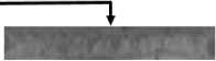
Normalized Iris

• 3.4.    Feature Extraction

  In 1996, Ojala et al. introduced the Local Binary Pattern technique to exploit the statistical and structural texture patterns [7, 40]. This work extends the original LBP based on image blocks concerning neighborhoods of different sizes and it is a relatively newer feature extraction method for remote iris recognition. It performs on local spatial patterns and grey scale contrast as well as counts various types of texture patterns, which are generated in the neighborhood of each pixel.

5	4	3
4	3	1
2	0	3

a

1	1	1
1		0
0	0	1

b

2»	21	22
27		23
2й	25	24

c

1	2	4
8		16
0	0	128

Binary Code: 11101001

Decimal Number: 143

d

Fig.3. Basic LBP operation on 3 x 3 pixel neighborhoods. a) Pixel values of the greyscale image, b) Binary pattern after thresholding S ( g_P - g_C ) , c) Binomial weight 2 ^P and d) Binary code to LBP decimal code.

This study considers only one block and shows how to extract LBP features as illustrated in Fig.3. Basically, the LBP descriptor labels the pixels using a complementary measure of local image contrast. The LBP label is a binary number defined for each pixel, where each bit is encoded by taking its difference from the center pixel g ( x , y ) at a given radius R . For this purpose, the coordinates of P neighbors g ( x , y )are first evaluated by a bilinear interpolation because they do not exactly fall on pixel values. Different radii and the number of pixels in the neighborhood are allowed as a result of bilinear interpolating on these pixel values. It is done with the help of sinus and cosines:

x p = x c + R cos(2 np / P ) &  y p = y c + R sin(2 np / P )

If gc (xc, yc) and gp with p = 0,1,2,...........P -1 are the gray values of the center pixel and its neighbor respectively, then the texture U in the local neighborhood of the center pixel may be defined by T = t(gc, go, gi,......gp-i). The P bit binary code is generated in the local neighborhood of each pixel by taking the difference of the center pixel for its P neighbor pixels one by one. The differences are influenced by scaling being invariant against grayscale shifts. Only the signs of the differences are taken into account for invariance to any monotonic grey scale transformations.

T - 1 ( S ( g 0 - g c ), S ( g 1 - g c ),............, S ( g p - 1 - g c ))

Where, S ( g_P - g_c ) is the thresholding function given by

S ( g p - g c ) =

¹ g p ^ g c

⁰ g p < g c

Secondly, the corresponding pixels S ( g_P - g_c )are multiplied by a binomial weight 2 P to convert the difference values into a distinctive LBP decimal code for a local neighborhood. This code characterizes the contextual information and spatial patterns of the local image texture around the center pixel. The decimal code is computed from P neighbors located on a circle of radius R of a grayscale image as follows:

p - 1

LBP p , r ( X c , y_c ) =2 S ( g p - g c )2 ^p p = 0

The total number of binary patterns with P neighbors is 2^P.

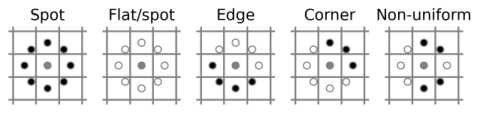
Fig.4. Examples of different texture primitives

Thirdly, the number of possible binary codes increases exponentially with larger neighborhoods. This can be limited using uniform patterns i.e., uniform appearance of LBP . These patterns only count once 2 bit-wise transitions from 0 to 1 or 1 to 0 in the circular P bit binary codes [11]. Some examples of uniform patterns for 8-bit binary code are 11111111, 00000000, 11001111, 00111100, and 11000111 but 11101110 is nonuniform for 6 transitions. The uniform and non-uniform local binary patterns are illustrated in Fig.4. As a result, the number of possible uniform patterns with U( x , y ) <  2 is P ( P -1) + 2 instead of the original 2 P for its P neighbors. Algebraically, the “uniformity” of a neighborhood is formulated by

U ( x , y ) = | S ( M p - 1 - M_c ) - S ( M 0 - M_c )| +2 | S ( M p - M_c ) - S ( M p - 1 - M_c )|

Finally, the remaining patterns withU( x , y ) >  2 are assigned a “miscellaneous” label, and a histogram with all possible labels is constructed for each block. The block histogram comprises of P ( P -1) + 3 .bins, where every bin includes a pattern and records the number of its appearances [41]. The histogram of these patterns i.e., also called labels forms a feature vector of the image. If L is the label of j th bin and n is the number of different labels, then the histogram of the labeled image f_l ( x , y ) can be written as

H i = 2 Im{ f, ( X , y ) = L ( i )}, i = 0,1,........., n - 1

x , y

I 1

Im( A) = |0

Ais true

A is false

The histogram contains information about the distribution of the local micro patterns, namely, spots, flats, lines, edges, and corners over the whole image [7, 41]. In order to retain spatial information, the image is divided into several blocks R 0 , R 1 , R 2,........... R m - 1 . The spatial histogram of j block is given by

Hi , j = 2 Im{ f ( x , y ) = L(i )},Im{( x , y ) e R j }, i = 0,1,........., n - 1, j = 0,1,........., m - 1

This histogram has three different levels of locality: (i) the labels contain information about the patterns at the pixel level, (ii) the labels are summed over a small block to extract spatial information at the regional level and (iii) the block histograms are concatenated to construct a global feature vector of the image.

• 3.5.    Classification

The K-Nearest Neighbor is regarded as one of the oldest and most used supervised distance-based machine learning algorithms due to its simplicity and low error rate [39]. Statistically, KNN is a lazy learner because it stores all the data instead of learning in training mode and performs only at the time of classification. It is also called nonparametric, which refers to making no underlying assumptions about the distribution of data.

All of the distance-based algorithms previously employ Euclidean metric for distance measurement. However, none investigates the effects of choosing different distance metrics. The following distance metrics are used to provide a comparative study of the performance of the KNN classifier. If x = ( x_Y , x ₂, x ₃, , x_n )and y = ( y_r , y ₂, y ₃, , y„ ) e R n be two feature vectors in a 2D plane, the below distance metrics are computed as follows:

Euclidean distance (Euci): This distance is the geometric extension of the Pythagorean theorem, which measures the length of a line segment between the corresponding coordinates of two points.

n

D Eucl ⁽ x , У ) =

I x n - у_и| = JZ ⁽ x j - y , ^{) 2}

i = 1

Minkowski distance (Mink): Minkowski distance is a generalized metric of order (οd) defined as L norm:

n

D Mink ( x , У ) = оА X ( x , - y ,)^od                                       (12)

i = 1

City Block distance (City): It is a special case of Minkowski distance where od = 1 . It computes absolute differences between a pair of vectors and then adds the difference consistently as

D City ^{( x} , y ) = Z| ^xj ^- У ,                                             ⁽¹³⁾

, = 1

Chebyshev distance (Cheb): Chebyshev distance is an expansion of Minkowski distance with od = » . The distance measures the greatest difference between any two vectors with one-dimensional coordinates. The formula to find the distance is:

D Ched ^{( x} , у ) = maxi x, ^- у,|                                           ⁽¹⁴⁾

Sokalsneath distance (Soka): It is the ratio of matches to non-matches. The distance computes the dissimilarity between two Boolean feature vectors x and y by

^DSoka ⁽ x , У ) =

2( C tf + C ft )

^CTT + ^{2( C}TF + ^CFT )

where, C_v is the number of occurrences of x [ k ] = u and y [ k ] = v for k >  n .

Cosine distance (Cosi): Cosine distance that is also known as angular distance, is computed by the subtraction of cosine similarity from numerical value one. Where the similarity is measured by the cosine of the angle between two attribute vectors in inner product space.

D CoA^x , у ) = ^{1 - cos} 0 = ^{1 -}

x • У xy

= 1 -

n

X , = 1 ^x, y ,

where, cosine similarity is x • y = || x||||y || cos 0 ^ cos 0 = x • y/||x||||y||

Correlation distance (Corr): Correlation distance is the measurement of association strength between non-linear random vectors of arbitrary. This distance is calculated from one minus the Pearson’s correlation coefficient of two attribute vectors

n

^D Corr ^{( x} , У ) = ^{1 -}

Z ^{( x} , ^{- x )(} У J ^- У ) . i = 1

nn

Z ⁽ x j - x ) JZ⁽ y J ^- y )

J =1   ^J         M / =1   ^J

Canberra distance (Canb): Canberra distance is a weighted form of L 1 norm, where the absolute value of differences between a pair of attribute vectors is divided by the absolute summation of attribute values before summing. It’s mostly applied to data scattered surrounding the origin.

n

D Canb ⁽ x , У ) = j

= 1

Braycurtis distance (Bray): In the field of biological sciences, Braycurtis distance has a robust monotonical relationship with ecological distance due to composition data. It sums the differences between two attribute vectors and finally, is standardized by their summed attribute values.

^DBray ⁽ x , У ) =

j и y j l ^1+^1

J =           j =

Jaccard distance (Jacc): The Jaccard distance measures the dissimilarity and diversity of feature vectors. The metric is attained by the subtraction of the Jaccard similarity index from one. Here, the Jaccard index calculates the similarity between the opposite binary vectors only.

^DJacc ⁽ x , У ) = ¹ -

j [ ( x j * У/ ) ^ ( ( x J * 0M У J * 0 ) )

^{j [ (} x j * 0H y j * 0 ) ]

4. Results and Discussion

All the experiments in this work are conducted on the largest long-range database CASIA-v4, which is a publicly accessible database for facial images at a distance. The Chinese Academy of Science’s Institute of Automation in China has released the biometric database [42]. The facial images are acquired at 3 meters away from the acquisition device under unconstrained environments using near-infrared imaging. The database makes up of 142 subjects including a total of 2,567 facial images. Since the human iris not only differ between identical twins but also between the left and right irises. We have separated all of the eye images from the facial images and attained 5,134 eye images. The separated eye images are included in different subjects belonging to the same person. We cannot separate a few eye images accurately from the facial images due to certain noises such as glasses, hairs, and reflections. Although most of the subjects have both regular and complicated images, the first 14 subjects have only regular eye images. The sample of NIR eye images from varied environmental challenges is illustrated in Fig.5. intending to increase the system performance and reliability of the classifier, we ignore the first 14 subjects in this evaluation. Randomly, we select a total of 3,041 images for training the classification models and 712 images for testing from the rest of each of the 128 subjects. The experiments are conducted using MATLAB R2018a (Intel core i5) and Python 3.7.

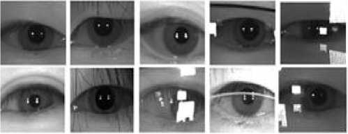
f ig .5. r egular and complicated images from casia- v 4 distance database [25]

The algorithm computes the distances between a pair of feature points and these distances are influenced by the measurement units. So, it is more convenient to make all the features (V) in the “same” scale and with the “same” distribution for computational simplicity. The min-max normalization formula is defined as follows:

у’ =(V -V ■ )/(V jj min   max

—

V ■ ) min

• 4.1.    Evaluation Metrics for Classification

There are several measurement techniques to evaluate the performance of a classifier. The most widely used statistical measures are average precision, recall, and F 1 –measure computation [34]. Specifically, accuracy indicates the overall performance of a classifier and it is computed as the ratio of the number of accurate classified images and the total number of test images.

Number of accurate classification Accuracy=

Number of all test images

The measurement systems are formed by the following to evaluate the classification performance of each class: (i) true positive (tp) : observation is positive (p) and predicted as true (t) ,(ii) true negative (tn) : observation is negative (n) and predicted as false (f) ,(ii) false negative (fn) : observation is positive (n) but predicted as false (f) ,(iv) false positive (fp) : observation is negative (p) but predicted as true (t) .

The following measures are computed to report the efficiency of multi-class classification problems.

1          tp j

Average Precision = — ^------ C j = i tp + fp ,

1          tp j

Average Recall = — ^------ C , = 1 tp , + fn ,

Precision x Recall

F i -meaure =2 x----------------

Precision x Recall

1                tn j

Accuracy = — ^-------------

C , = 1 tp , + tn , + fp + fn ,

Where, C is the number of classes; tp j , fn j , fp j , and tn j are the number of true positive, false negative, false positive and true negative for class j respectively. These measures are generated from the confusion matrix that visualizes the classification outcomes.

• 4.2.    Performance Evaluation

The performances of each distance metric and texture descriptor are compared to the indicators, namely, accuracy, F 1 -measure, recall, and precision values of the confusion matrix. The reported results in Table 1 are attained by customizing some parameters and experimental setups.

Table 1. Performance measure of distance metrics using LBP features.

Distance Metrics	Average Precision	Average Recall	F 1 -measure	Accuracy (%)
Euclidean distance	0.8620	0.8547	0.8417	0.8677
Minkowski distance	0.8620	0.8547	0.8417	0.8677
City Block distance	0.8804	0.8896	0.8729	0.9015
Canberra distance	0.9281	0.9049	0.9038	0.9282
Braycurtis distance	0.9427	0.9342	0.9301	0.9465
Chebychev distance	0.6275	0.5803	0.5591	0.5864
Sokalsneath distance	0.9209	0.9130	0.9051	0.9282
Cosine distance	0.8949	0.8860	0.8766	0.8973
Correlation distance	0.8912	0.8811	0.8723	0.8917
Jaccard distance	0.9209	0.9130	0.9051	0.9282

The Braycurtis distance acquires the highest average precision (0.9427), average recall (0.9342), F 1 -measure (0.9301), and accuracy of (94.64%), which is significantly better than other distances as enlisted in Table 1. Even though it achieves around 7% improvement over than most widely used Euclidean distance. It is experimented and investigated by Arnab et al. in [33] that the use of distance metrics depends on feature properties and the way to handle them. For example, if a bunch of zeros aren’t true absences in features, it will be better to use Euclidean distance. However, the LBP features are categorical or composition data as shown in Fig.13, and have a bunch of zeros for minmax normalization as mentioned in the sub-section 4.3. Dealing with composition data, the framework shows excellence in classification with Braycurtis distance over other distance metrics.

Table 2. Different gradient feature-based recognition accuracies.

Feature Descriptors	Average Precision	Average Recall	F 1 -measure	Accuracy (%)
u 2 LBP b	0.9427	0.9342	0.9301	0.9465
ri LBP g	0.8850	0.8607	0.8561	0.8790
riu 2 LBP g	0.8354	0.8232	0.8130	0.8410
u 2 LBP g	0.8589	0.8217	0.8150	0.8354
u 2 LBP f	0.7472	0.7313	0.7083	0.7369
u 2 LBP s	0.7100	0.6756	0.6575	0.6821
u 2 LBP n	0.6896	0.6566	0.6366	0.6638

Additionally, we apply the uniform ( u 2 ), rotation invariant ( ri ) and uniform rotated invariant ( riu 2 ) patterns on the local binary features to retrieve the shapes of local iris texture. The classification accuracies are 94.65% for u 2 , 87.90% for ri and 84.10% for riu 2 patterns and reveal that uniform patterns extract most of the iris patterns. The rotation invariant and uniform rotated invariant patterns are also extracted from iris patterns, which do not contain enough spatial information for these biometric identifications. Then the discriminatory power of uniform u 2 LBP b is compared to LBP n except block descriptor, fuzzy LBP f , gradient LBP g and shift LBP s to show its robustness against any monotonic grey scale transformations caused by the real-time environmental changes. In these cases, similar experimental setups are followed to KNN classifier with Braycurtis distance. Theu 2 LBP descriptor improves classification performance by around 28% significantly after applying block descriptor on the experimental database. Table 2 shows that the outcome of uniform patterns u 2 LBP b is the highest possible result compared to the u 2 LBP g , u 2 LBP f , u 2 LBP s , and u 2 LBP n descriptors.

The reason behind the performance ofu 2 LBP b is the better combination of machine learning techniques. Apart from this, the iris patterns are invariant to monotonic grayscale changes. In most real-time environmental images, these changes occur frequently due to varying levels of illumination as seen in Fig.5. In contrast, u 2 LBP b is robust to the monotonic gray-scale transformations and deals with local image contrast more effectively than other global descriptors. Furthermore, the block descriptor enhances the potentiality of extracting uniform iris patterns with local spatial information, which are the dominant features of iris textures. The above factors influence the classification performance significantly.

• 4.3.    Performance Study

We investigate the influence of setting various parameters and conclude that block descriptor, optimal value of radius, neighbor points and reliable distance metric are all important for promising performance. For ROC curves, the false positive rate (FPR) against the true positive rate (TPR) is computed with classification thresholds to visualize the diagnostic ability of the classifier by changing various parameters sequentially. The closer curve to the top-left corner indicates reliable performance. The description and analysis of the simulated results are displayed graphically and in tabular form in the following subsections.

Sliding Window: To assess the performance of block descriptors, initially we adopt different LBP operators in windows of varying size. The window variation causes difficulty in feature extraction and greatly affects the classification results. Fig.6 reports that the sliding window of72 x 72 pixels produce a substantial amount of context to retrieve micro patterns. The performance of the window 64 x 64 is similar to the window 72 x 72 but reduces recognition accuracy by 0.84% on the overall performance. The window 32 x 32 implements very fast with the lowest accuracy due to not having sufficient contextual and spatial information, whereas the other window size 128 x 128 performs with high computational cost.

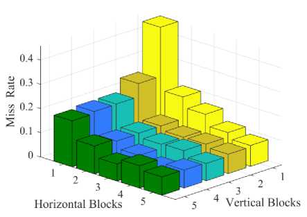
Fig.6. Window detection for LBP operator

0.6-

0.4

'                             ■ ■ ' 32x32 (AUC=0.97)

Q 2 J                           ■ ■ ■ 64x64 (AUC=0.98)

'  '                           ■■' 72x72 (AUC=0.99)

;                             ■ ■ ' 128x128 (AUC= 0.98)

• 0.0 -----------------.------------------.------------------>------------------>-----------------

  0.000     0.005     0.010     0.015     0.0200.025

0.8

False Positive Rate

Fig.7. Effect of block size on miss classification rate

Block Descriptor: In this study, the performance of the texture descriptor inextricably depends on the choice of blocks. The small image blocks not only extract the spatial information but also handle the local illumination changes. We follow several blocks along the horizontal and vertical directions to capture a large scale the significance of local pixels. The miss classification rate i.e., miss rate (%) is illustrated in Fig.7 with different block sizes. Most of the blocks perform equally and the3 x 4,3 x 5, and 5 x 3 blocks of 3 x 3 neighborhood pixels show also good performance among them as depicted in Fig.8. However, the 1 x 1 block provides the lowest performance with high dimensional feature vectors. In particular, 4 x 4 square block is most effective for retrieving uniform LBPs because of having enormous pattern variability in iris texture.

l.o -

ID

ID

0.6

ID

0.4

0.2

• ■    R=1 (AUC= 0.97)

• ■    ' R=2 (AUC= 0.98)

• ■    । R=3 (AUC= 0.98)

. R=4 {AUC= 0.99)

• ■    i R=5 {AUC= 0.99)

0.0 4— 0.00 0.01 0.02 0.03 0.04 0.05

False Positive Rate

Fig.8. Different Radius of neighborhood circle for feature extraction

Hl ф 0.6

'7

0.2

0.0 4----------.—

0.00       0.01

• ■    ■ ' P=5 (AUC= 0.96)

• ■    ■ । P=6 (AUC= 0.96)

• ■    ■ ■ P=7 (AUC= 0.97)

P=8 {AUC= 0.99)

• ■    . . P=9 (AUC= 0.97)

• ■    ■ । P=10 (AUC= 0.96)

0.02       0.03       0.04       0.05

False Positive Rate

• Fig.9.    Number of neighbor points on the circle for LBP features

0.8-"

Radius of Circular Neighbors: The LBP descriptor is highly sensitive to its neighbors and the radius of the neighborhood as well as the total number of pixels comprising the image. The overall performance of the model is greatly affected by the size of neighborhood circles. Therefore, it is a rather challenging task to set a threshold value of radius R . Actually, the radius defines the number of neighbor points around the center pixel. The feature retrieval performance increases with the increased radius up to 4 and the performance falls dramatically at the radius 4. The effect of changing radius R from 1 to 5 has been shown in Fig.8. It is observed that the texture method exhibits poor performance at radius 1. On the other hand, the discriminative power of the proposed LBP feature descriptor is considerable when R is equal to 4 in the case of 8 circular neighbors.

Number of Circular Neighbors: To find out the optimal number of circular neighbor points is one of the most challenging tasks. Since the shape of regional iris patterns is highly connected to its neighbors. We plot the miss-classification rate concerning vertical and horizontal blocks and carry out the experiments several times to optimize the number of neighbors points P. The chosen of P neighbors from 5 to 10 leads to obtaining various performances as shown in Fig.9. The highest performance can be obtained at 8 neighbor points and radius 4 of neighborhood without other competitive neighbor points. The local shapes are neglected with larger neighborhoods. Consequently, the classification performances are decreased because of the loss of spatial information.

Number of K Neighbors: Informative features are the pre-requisition of learning the KNN model that addresses the missing values, normalization, and lower dimensionality of features. Choosing the value of K is quite challenging. A small value leads to noise and increases the impact of outliers on the overall outcomes. Large values cause perplexity, and high computational costs as well as defeat the basic concept of the KNN algorithm. We observe from Fig. 10 that there is no optimal value of K , which performs equally well for all distances and descriptors. Changing the K value from 2 to 5 provides various classification performances and shows that neighboring points get priority over the farther points to classify the unknown objects. Additionally, we notice that the best performance can be achieved with 3 nearest neighbors for the extracted local binary features.

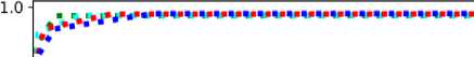
^     '                                  ■ ■ ' K=2 (AUC=0.99)

0 2 J                                ■ ■ ■ K=3 (AUC=0.99)

’   ■                                     . . । K=4 (AUC=0.99)

;                                   ■ ■ ' K=5 (AUC=0.99)

0.0 4----------------,----------------.----------------r----------------,---------------- 0.000      0.005      0.010      0.015      0.0200.025

False Positive Rate

• Fig.10.    Effects of selecting K as nearest neighbors

  
  
  

  1.0

  0.8

  0.6

  0.4

  0.2

  0.0

  
  

*?Д^>>^^^ДДЛМьЫьХХХХХХХМИ1ММХХ

• ■    ■ ¹ Euclidean distance (AUC= 0.97)

• ■    ■ ¹ Minkowski distance (AUC= 0.97)

Braycurtis distance (AUC= 0.99)

• ■    ■ ¹ Canberra distance (AUC= 0.98)

• ■    ■ ¹ City Block distance (AUC= 0.98)

Chebychev distance (AUC= 0.88)

• ■    ■ ¹ Jaccard distance(AUC= 0.99}

• ■    ■ ' Sokalsneath distance (AUC= 0.98)

• ■    ■ ¹ Cosine distance (AUC= 0.97)

• ■    ■ ¹ Correlation distance (AUC= 0.97)

  0.00       0.01       0.02       0.03       0.04       0.05

  
  

• 4.4 Discussion and Statistical Analysis

  This sub-section discusses the limitations concerning the experimental database. The robustness and stability of a machine learning algorithm will be increased with higher values of precision, recall and F 1 -measure and accuracy, which are measured from the confusion matrix. Though the framework provides better accuracy for near-infrared images, it cannot recognize complicated iris images accurately due to having several challenges in a few subjects. The range of test and training features varies in each subject despite applying the min-max normalization technique. For example, a common feature distribution of training and test images is shown in Fig.12. Whereas, the range of the training features is (0; 1), for which the values of mean, median, and mode are 0.0502, 0.0078 and 0 respectively; and the standard deviation is 0.1191. The range for the test features is (0; 1), for which the values of mean, median, mode, and standard deviation are 0.0465, 0.0079, 0, and 0.1125 respectively.

False Positive Rate

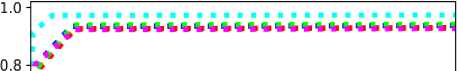
Fig.11. Performance of different distance metrics

Performance of Distance Metrics: A good distance metric helps to enhance the performance of classification, clustering, and information retrieval processes greatly. We evaluate the performances of the distance metrics using confusion matrix and ROC curves in case of exploiting LBP features. The experimental results in Table 1 show that Jaccard, Spearman, Braycurtis, and Canberra distances perform almost well, while Canberra distance reduces performance by 2% and the performance of Sokalsneath is similar to Jaccard distance for the local uniform binary features. Though the performances of Euclidean and Minkowski distances are equal, Euclidean distance performs noticeably better than Minkowski distance in Fig.11. Chebychev distance always shows poor performance with increased computational simplicity. It is also observed that the precision, recall and F1 -measure are different for Correlation and Cosine distances despite having almost equal accuracy.

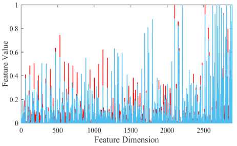
Fig.12. Train and test feature distributions within a common subject randomly

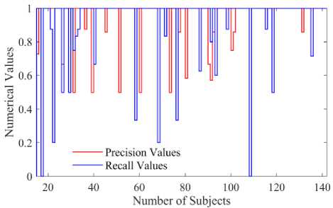
Fig.13. Subject-based precision value curves

It is visible that the LBP b features are not distributed uniformly and have non-linearity, which is the basic assumption of the nearest classifier. However, the levels of non-linearity are investigated in most of the subjects, and reported that few subjects have more non-linearity that creates complexity for iris recognition. It is also clarified that most of the captured images of these subjects have reflections, glasses, hair, or other noisy factors. Due to having many non-linear features than the ratio, the proposed approach cannot attain the highest accuracy and the classification performance reduces quite a lot of these subjects.

The precision and recall curves are plotted to visualize how the imbalanced dataset affects classifier performance within each subject. The 19 subjects for precision and 21 subjects for recall curves cannot attain the highest value. It can be observed from Fig.13 that the lowest recall value of the 17th and 108th subjects is 0.0, which means that the images cannot correctly identify belonging to their subjects. The lowest precision value of 31th, 39th, 51th, 60th, 73th subject is 0.50. Noticeably, the lower precision values have the corresponding higher recall values and vice versa. It shows that more complicated and irregular images are contained in the following subjects. In practice, these 40 subjects have different types of noisy images. As a result, the system cannot acquire 100% accuracy due to having illumination variations and flat areas in these subjects. A precision-recall curve helps to visualize how threshold affects classifier performance.

Table 3 shows the recognition performances of the framework compared with earlier approaches. It should not compare the obtained results explicitly with others because these methods were conducted on various types of databases with different distributions like subjects, train, and test images. Even most of the authors employ a small number of test and training images to conduct their experiments. These subjects have only regular and ideal images at a close distance.

Table 3. Performance evaluation with existing competitive methods.

Distance-based Different Approaches	Recognition Rate (%)
Symlet wavelet with Spearman distance, Arnab et al. [39]	78.38 %
LS and LBP with Manhattan distance, Roy et al. [22]	81.45 %
1D LG and Hamming distance, Masek et al. [16]	83.92 %
Uniform LBP and Euclidean distance, Li et al. [23]	84.77 %
LBP and Euclidean distance, Patil et al. [24]	84.88 %
LaGaF, and Normalized correlation, Wildes et al. [13]	86.49 %
CNN and Euclidean distance, Ali et al. [43]	86.96 %
Monogenic LG and Hamming distance, Chan et al. [44]	90.43 %
Uniform LBP and Bhattacharyya distance, Huo et al. [26]	90.79 %
GLAC and correlation distance, Ripon et al. [33]	91.84 %
Uniform LBP and Braycurtis distance (Proposed)	94.65 %

For instance, Tan et al. made use of 935 images from the near-infrared database [42]. Subjects 1-10 are considered for training images to learn the models. In contrast, the test images are taken from the first 8 left iris images of the rest 11-141 subjects to evaluate recognition performance. Their experimental outcomes were reported as 94.66% in [45] and 95.00% in [46] respectively. In contrast, our approach has been evaluated on a large number of 3,753 eye images with 3,041 training images and 712 testing images from 128 subjects. We avoid the first 14 subjects for regular images to prove the robustness of LBP b against various practical conditions like illumination changes, low contrast, occlusions, etc. However, the extended feature descriptor and distance classifier provide the highest accuracy from long-range iris recognition and have the potential to overcome the existing issues. The comparison with prior conventional algorithms demonstrates that the above biometric framework is more practical for human identification than other global texture and distance-based approaches.

5.    Conclusion and Future Work

In this work, we present a discriminative and effective local texture descriptor for distant iris recognition under unconstrained environments. The textures of the iris regions are retrieved locally with the help of LBPs , while the macrostructure of the iris image is recovered by the concatenation of regional histograms. It is observed that uniform patterns account for most of the iris patterns and reflect the statistical properties of the local micro patterns, such as edges, spots, and flat areas over the iris texture. The experimental outcomes demonstrate that the performance of the classifier not only depends on distance metrics but also on the quality of features. Also, the LBP texture features are invariant to monotonic gray-scale changes resulting in illumination variations. Consequently, the Braycurtis distance classifier attains the highest possible accuracy (94.65%) compared to other distance metrics. Although the machine learning algorithm shows its superior performance on one of the most challenging databases, the descriptor and classifier have the following drawbacks: (i) The bit-wise comparison is affected by noise pixels due to its small spatial support. (ii) The larger-scale structures are not captured completely from the local 3 x 3 neighborhood that may be dominant features of iris patterns. (iii) The length of feature vectors increases with a large number of image blocks and slow classification performance with high computational cost. In contrast, the spatial information is lost significantly with a larger image block. (iv) It fails to prove its robustness on flat region texture because of having no intensity differences. (v)The nearest classifier becomes biased towards the majority of instances of training features. For future studies, it is more important to focus on iris image pre-processing like noise removal, iris segmentation, and normalization than feature extraction. Many ways could enhance the system performance, for instance, the influence of local noise pixels could be suppressed considering gradient local autocorrelations on the blocked base LBP . Using several blocks with weights according to their spatial positions emphasizes on LBPs that contain the most relevant texture information. A possible way is to follow dimensionality reduction techniques. Another possibility is to employ a proximity-weighted evidential scheme for compensation for the bias towards the majority of instances in training space for the nearest classification. The comparative studies suggest selecting the most effective distance metric for distancebased approaches according to the quality of features. However, the framework presented here applies to the other object recognition tasks that have enormous pattern variability with a high degree of randomness and uniqueness like iris texture.

Acknowledgment

This work was supported by the National Science and Technology (NST), Government of the People’s Republic Bangladesh. We also acknowledge the Institute of Automation (Chinese Academy of Science, China) for the contributions of the database employed in this work.