Block Texture Pattern Detection Based on Smoothness and Complexity of Neighborhood Pixels

Published Online April 2014 in MECS DOI: 10.5815/ijigsp.2014.05.01

Texture modeling is an active area and has been studied over the past three decades. In this subject, depending on the size and the spatial arrangement of the texture elements, texture images are grouped into macro, micro, periodic, aperiodic, coarse, fine, regular, random, weak, strong, stochastic, non-stochastic, deterministic and non-deterministic textures [1]. Also, most of the texture modeling techniques can be grouped into either statistical or structural methods [2]. In this paper, our method is based on statistical techniques. Some well-known statistical methods includes spatial gray-level cooccurrence matrices [3], Gaussian-Markov random field [4], Fourier power spectrum, gray-level run-length, graylevel difference matrices [5], texture energy measures [6], fuzzy techniques [7, 8]. The other newest texture models are stand wavelet, Gabor filter and fractal dimension which are highly addressed in [9, 10, 11, 12 and 13].

The degree of smoothness and complexity in a block texture pattern has a key role in image processing and computer vision. Complexity of images is not only been used in image recognizers [14], but also has been used by content-based image retrieval (CBIR) [15], data hiding algorithms [16], and detecting the different geographic region such as old-growth forest ecosystem [17]. In addition, detecting a region in images with different measure of smoothness and roughness is important for detecting and removing noises in images [18]. Also, knowing the measure of smoothness in different region of an image can improve the watermarking and steganography algorithms which hide secret messages in spatial domain of an image. For example, as it will be illustrated in this paper, it can effectively improve the performance of Pixel Value Differencing (PVD) algorithm.

In this paper, firstly, the definition of smoothness and complexity are discussed, and a new categorization of texture is defined in Section 2. Then, in Section 3 we develop a new statistical method for categorizing a block texture based on smoothness and complexity measures. This method is mainly based on calculating the difference between neighborhood pixels and the variance of the elements in a BxB block. In Section 4, results of proposed algorithm are shown, which is implemented with MATLAB. The results show that this method can determine the texture blocks base on smoothness and complexity of an image with high confidence. Next, the effects of this texture classification are illustrated on three different steganography algorithms in spatial domain which are include Least Significant Bit (LSB) [19], Pixel Value Differencing (PVD) [20] and a steganography algorithm based on Matrix Pattern (MP) [21].

• II.    SMOOTHNESS AND COMPLEXITY

In this section we discuss about two measures of smoothness and complexity in details.

In an image, a smooth region is defined as a uniform area where the difference between two adjacent pixels is small. Usually, an image has several uniform smooth regions, which are separated from each other by some edges. In other words, edges identify the boundaries between areas in an image, which can help for segmentation and object recognition [22].

The efficiency and performance of many image processing and computer vision algorithms and methods can be improved if the degree of smoothness in the texture can be accurately and efficiently identified. For example, PVD [20], a well-known steganography algorithm, hides less data in smooth areas in than edge regions, and it has been shown that finding the areas with the smaller smoothness degrees enhances the performance of the algorithm.

Complexity of binary blocks has been defined by Kawaguchi et al. [23] as the number of changes between black and white pixels in vertical and horizontal directions. As an illustration, in an 8x8 block, the maximum possible changes are 112 in a chessboard pattern. This measure has been used in their steganography algorithm for hiding the data in the complex blocks. In this paper, complexity degree is applied similarly, but on the gray-level of images.

In this section, we classify block texture patterns to four major groups based on their smoothness and complexity values:

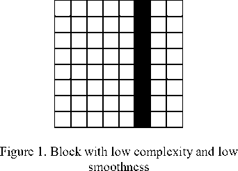
• •    Edge (low smoothness) with no complexity: A block is in this class if the total number of difference between neighborhood pixels of the block is not high, i.e. the complexity is low; but an edge drastically changes the neighborhoods in a part of block, i.e. low smoothness. Figure 1 shows a sample of black and white block with low smoothness and no complexity.

  

• •    Smoothness with no complexity: In this class of blocks, the texture is plain and neighborhood pixels are similar to each other, i.e. the block has high smoothness. Also, the values of most of neighborhood pixels are the same; thus, the block has no complexity. A complete black or white block is an example of smoothness with no complexity.

• •    Smoothness with high complexity: This class of blocks may be seen in gray-scale images. In this class of blocks, the difference between neighborhood pixels is not high, i.e. the texture is smooth; on the other hand, the values of neighborhood pixels are not the same, i.e. the complexity of the block is high. Note that in smooth areas, it is possible that neighborhood pixels do not be the same. This mild difference between every neighborhood pixel makes the texture both complex and smooth. In our classification, we name the forth group as the perfect case of “fine texture in smooth region”.

“Fine texture” has been defined by Arivazhagan et al. [1] as a texture that its primitives are small (number of pixels which are use for a main shape of texture are less) while the tonal difference between neighborhood primitives is large. In contrast, in a coarse texture block, the primitives are larger and consist of several pixels [1, 24]. Figure 3 [1] shows the difference between fine and coarse textures.

• Edge (low smoothness) with high complexity:

This class includes blocks that their neighborhood pixels are highly different. In other words, both edge and complexity measures are high. A block of this kind, in the best case would be a fine texture that has been described by Arivazhagan et al. [1]. Figure 2 illustrates a

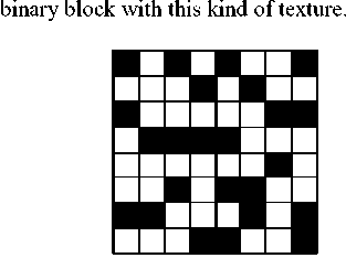
Figure 2. Block with high complexity and low smoothness

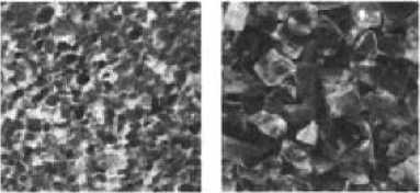
Figure 3. a) Fine texture b) Coarse texture

As you may notice, it seems that there is a conflict between definition of fine texture and smooth region. In a fine texture, neighborhood pixels are highly different, while in a smooth area the pixels are similar to each other. Finding such area would be a challenge. To determine fine textures in a smooth region, we extract some blocks in the smooth region of image that its primary neighborhood pixels (by primary neighborhood pixels, we mean 8 neighbors pixels) be different enough. In other words, comparing to the uniformity of region, the deference between primary neighborhood pixels should be high and do not be the same as each other.

• III.    METHOD

For grouping blocks in an image, at first, RGB layers of image are separated, then, the brightness of the whole image is computed by (1) [25, 26].

Brig ℎ tness ( P ( r , g , b ) ) =(0․2126∗ r ) + (0․7152 ∗ g ) + (0․0722∗ b )                                (1)

Then, the image is divided to the BxB blocks with fix sizes. The degrees of smoothness and complexity of blocks texture are calculated by applying the following steps:

At first, for identifying the smoothness degree of blocks, the variance of gray-level of image brightness is computed. Equations (2) and (3) show the formula for calculating the variance of BxB block.

Pavg =(∑ BxB p ( i )⁄ BxB )                           (2)

In (2), the two-dimensional block is transformed to a one-dimensional block named “P” .

Variance =    ∑f=l ( p ( i )- ^avg )²                 (3)

Having more variance in each BxB block shows that the block is less smooth and vice versa.

Several algorithms have been proposed for obtaining the complexity of a binary block. For example, Kawaguchi et al. [23] determined the complexity by calculating the number of changes between black and white in vertical and horizontal dimensions. In this paper, we have improved their algorithm. Note that, we are trying to identify the complexity of gray blocks and not binary (black and white) blocks. For that, we propose an algorithm that modifies the gray-level image to a binary one by averaging each block using (2). Then, each pixel in the block is compared with the average, if it is equal to or higher than the average, it is modified to one (white), and if it is lowers than the average, it is set to zero (black). Finally, the numbers of changes in the block from black to white and vice versa is counted. Figure 4 shows the counting step for an 8x8 block in both vertical and horizontal orders as well as in diametrical (from upper left corner and upper right corner) order.

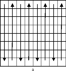
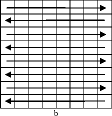
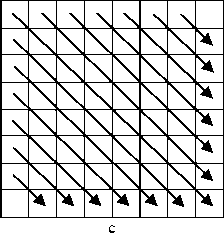
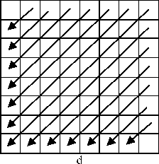
Figure 4. a) Vertical counting b) Horizontal counting c) Diametrical counting from upper left d) Diametrical counting from upper right

For estimating the complexity of each BxB block, as mentioned before, first the block is transforms to a binary block, then, the number of changes from a pixel to another one is calculated in both vertical and horizontal as well diametrical orders. Being divided by the maximum possible changes for that order normalizes the obtained numbers.

Equations (4) and (5) are used for calculating the complexity in vertical and horizontal orders. As shown by Kawaguchi et al. [23], the maximum possible changes in a square block in any of vertical and horizontal is equal to B*(B-1) .

Ver = ⁄ В ∗( В -1)                           (4)

Ног =  ⁄ В ∗( В -1)                          (5)

In (4) “V” is the number of changes in vertical order and in (5) “H” shows the number of changes in horizontal order.

Here, we show the maximum changes that is possible to occur in the diametrical order for a BxB block:

To calculate the maximum number of changes when the pixels in the block are traversed in diametrical order, we need to find the maximum number of changes in all the diameters. A BxB block has (2*B)-1 diameters with lengths of B, B-1, …, 2. The main diameter in a BxB block has B consecutive pixels and the maximum possible pixel change between them is (B-1). The next two longest diameters include (B-1) pixels with maximum (B-2) possible changes. As it has been illustrated in Figure 5, an 8x8 block, the main diameter has 8 pixels with maximum 7 possible changes, and the next two longest diameters in green have 7 pixels with 6 possible changes. And obviously, the two shortest diameters pixels, in red, maximum can have only one possible change from one pixel to another.

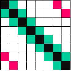
Figure 5. A sample 8x8 block by different diameter size

Thus, the formula for calculating the maximum possible changes in diametrical order is:

Max^tametric=(В-1)+ 2∗∑t=i i(6)

Equation (7) is always true [27]:

yi     =

∑=

For computing the complexity of the whole block, the value of all of the measures: “ Ver”, “Hor” , “ Dia1” and “ Dia2” are sum upped. Then, the result is normalized by being divided by the maximum possible change in the entire block. For calculating the maximum possible changes in a block, we cannot simply sum up all of the maximum possible changes in the vertical, horizontal and two diametrical orders. Because these measures are not independent, and it is impossible to have a pattern which has the maximum changes of all four measures at the same time. Kawaguchi et al. [23] have shown that the chessboard pattern has the maximum possible changes in vertical and horizontal ways. Figure 6 shows an 8x8 block with chessboard pattern.

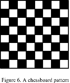
You can see although chessboard pattern shows the maximum possible changes in vertical and horizontal orders, there is no pixel change in any of the diametrical orders. In other words, the maximum possible change in this kind of pattern can be calculated with (12).

M aX_Ch.essboard =2∗( В ∗( В -1)) (12)

By using (7) in (6), we get (8).

MdX diametric =( В -1)+2∗(

( в -2)∗( в -1)

)

A pattern includes the maximum pixel changes in the diametric orders, if it has a black and white row or column in decussate. Figure 7 indicates two examples of 8x8 patterns that have the maximum possible changes in the diametric orders. In addition, these patterns show the most possible changes in vertical or horizontal ways.

By simplifying (8), equation (9) is achieved.

М о.Хд[_ате1;г[_С = ( В -1)+( В -2)∗( В -1)=

( В -1)²                                          (9)

The maximum number of possible changes for the other set of diameters, the ones started from upper right corner, is equal to (B-1)² as well.

Thus, the complexity for diametrical orders can be computed by (10) and (11):

Dia,1=Diametrical сℎanges(upper left)⁄(В-1)2

Dia2=Diametrical cℎanges(upper rigℎt)⁄(В-1)2

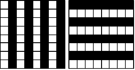
Figure 7. Decussate patterns with high changes in diametrical ways

Equation (13) computes the number of pixel change in patterns shown in Figure 7.

MttXdecussate = ∗( В -1)+2∗( В -1)² (13)

Equation (14) shows the subtraction of (13) from (12). If this value becomes positive for any block, it means the maximum possible change in decussate pattern is more than the chessboard pattern and vice a verse. It is obvious that the least block size is 2x2.

А=            - М CLXCh,essboard =   -3в+2

for В ≥2 → А ≥0                         (14)

As (14) shows, the value of “ A” for each block size is positive or zero; thus the possible changes in decussate pattern is more than chessboard pattern, and in worse case they are equal.

Notice that patterns without equal number of black and white pixels have less number of pixel changes, and random patterns with equal black and white pixels cannot have more changes than decussate patterns. Thus, for normalizing the complexity of a block, the sum of vertical, horizontal and both diametrical measures are divided by the maximum possible changes calculated by (13).

If the number of changes in one of the vertical, horizontal or any of the two diametrical is zero (or near zero), but the amount of changes in the whole block is high, it means that the block has a consistent pattern. As Figure 8 shows, the chessboard pattern in left does not have any changes in diametrical ways and block in right does not have any changes in vertical order. Patterns in Figure 6 and Figure 7 have this trait as well.

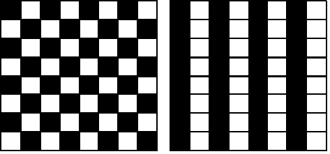
Figure 8. Two blocks with high change with consistent pattern

Our method for detecting the complexity of binary blocks is more efficient than the method used in BPCS algorithm [23], because for calculating the new complexity measure, the changes between black and white pixels in diametrical orders are considered as well.

• IV.    IMPLEMENTATION

We applied MATLAB to implement and evaluate our proposed algorithm. The inputs to the algorithm are: an image, size of BxB blocks, the threshold values for changing parameters in vertical, horizontal, and diametrical measures, and the threshold values for total changes between primary neighborhood pixels. The results indicate that this method can successfully detect the type of texture of any of the blocks.

Figure 9.a shows an image that includes blocks with edge (low smoothness) and low complexity. The size of each block in this image is 64x64, 4096 pixels in each block. The selected blocks are those in yellow squares.

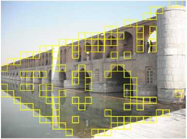
Figure 9.a. Blocks with edge and no complexity

One of the chosen blocks is illustrated in RGB, gray and binary scales in Figure 9.b. Notice that the binary image is created by comparing each pixel with the average of pixels in gray-scale format.

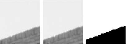
Figure 9.b. Block with edge and low complexity

In Figure 10.a, the blocks with edge and high complexity are shown in yellow squares.

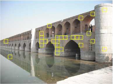
Figure 10.a. Blocks by edge and high complexity

One of the selected blocks is shown in Figure 10.b.

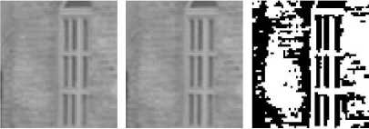
Figure 10.b. A block with edge and high complexity

Figure 11.a indicates some blocks with high smoothness and low complexity measures in yellow squares.

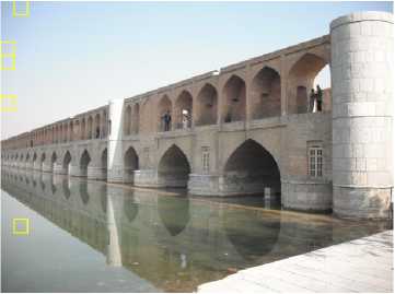
Figure 11.a. Blocks by high smoothness and low complexity

Figure 11.b shows a chosen block in RGB, the grayscale and the binary format.

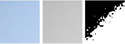
Figure 11.b. A block with high smoothness and low complexity

The studied image does not have appropriate blocks with high smoothness and high complexity. Figure 12.a shows another image and some selected 64x64 blocks with the high smoothness and complexity.

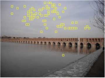
Figure 12.a. Blocks by high smoothness and high complexity

Figure 12.b. illustrates the RGB, the gray-scale level and the binary layout of a selected block.

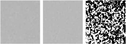
Figure 12.b. A sample of high smoothness and high complexity

The enlarged gray-level images of blocks show the degree of smoothness, and the binary images of them show the complexity of blocks’ texture patterns. The selected block in Figure 9.b has edge shown in gray-level block with no complexity between its neighborhoods’ pixels which is indicated in binary block. Also, Figure 10.b has high edge and high complexity. The expanded block in Figure 11.b has high smoothness and uniformity in the gray-level block, and low complexity shown in black and white. Finally, the enlarged block in Figure 12.b, an example of fine texture in smooth area, has high smoothness while its pixels in gray-level format are similar, but not the same.

• V.    APPLICATIONS

Detecting the smoothness and complexity of images could be vital for image processing applications including data hiding. In data hiding algorithm, which images are used as covers for secret messages, these parameters have a key roles for detecting the best region for hiding secrets. A well-known algorithm, PVD, is more efficient when it can hide data in an area within edges [20, 28]. In addition, the new matrix pattern based steganography system presented earlier by the authors can produce matrix patterns faster in the blocks of image with high complexity, and it can be used for assigning more parts of the blocks of image for inserting secret message [21]. Moreover, the algorithm presented in that article calculates the difference between the neighborhoods’ pixels to produce a “matrix pattern” and distribute it through the whole block. Thus, in the presented algorithm [21], the best block texture patterns for data hiding may be those having both high smoothness and complexity, as well as fine texture in smooth area. On the other hand, LSB, the most well-known data hiding algorithm in spatial domain, can be used in different texture patterns and gets good results. To increase the hiding capacity, steganography based LSB methods can select smooth region while other spatial domain algorithms such as PVD can use the remaining region of the image [29, 30 and 31].

For comparing the results of different BTPs, the effect of four block texture patterns which were discussed in pervious sections, are implemented and shown in three steganography algorithms, namely LSB, PVD and matrix pattern (MP). For this purpose, 2000 blocks of 64x64 sizes are selected for each type of the BTPs introduced earlier. Then, the maximum possible data are hidden in the total of 8000 blocks with all three different steganography algorithms.

Next, both capacity and transparency are compared with each other. Transparency is calculated using peak signal to noise ratio (PSNR) of cover as well as stego-blocks.

In order to calculate PSNR, firstly, we should derive the brightness with equation (1). Then, we compute mean square error (MSE) of the brightness of cover image and stego-image using the following equation.

MSE = ^П- ^T= г [Srighmess (/(, j) -Brightness (S(iJ)-)]                            (15)

In this equation “ n” and “ m” are the column size and row size of the images, respectively. Note that, “I” refers to the cover image and “S” refers to the stego-image [21]. Finally, PSNR is calculated with (16).

PSNR УД^О^УУ

As mentioned earlier, PSNR measures transparency in an image. If PSNR value becomes more than 30, it shows that the changes in the image could not be identified by human eye easily [28, 32]; and thus it has a “good” transparency.

Results of the each steganography algorithm base on each BTP classification are illustrated in Table I. In this table “E_S” , “E_C” , “S_C” and “S_S” refer to different BTPs including “edge and simple”, “edge and complex”, “smooth and complex”, and “smooth and simple”. In addition, the values in capacity rows show the number of characters that can be hidden with these algorithms.

Specifically, Table I shows the effect of each BTP classification on LSB, PVD and MP algorithms.

TABLE I. Results of LSB, PVD and Matrix pattern on different BTPs

Metho d	Measure Parameter s	E_S	E_C	S_C	S_S
LSB [19]	Capacity	102400 0	102400 0	102400 0	102400 0
	PSNR	43.6074	40.72	44.9516	51.1609
PVD [20]	Capacity	149996 3	184376 1	153830 4	107138 7
	PSNR	40.2568	35.0492	42.0444	44.6373
MP [21]	Capacity	874514	972982	100914 6	223133
	PSNR	47.6337	39.7529	52.9201	59.737

Table I indicates that for LSB method, not only capacity in different BTPs is the same, but also they have higher PSNR than PSNR=30. It is obvious that the capacity has no relationship with different BTPs. This is not true for transparency. Although transparencies of all of the BTPs in this steganography method are more than 30, “ S_S” has the best transparency result.

The other two steganography algorithms of PVD and MP do not follow the same results. Table I illustrates that for PVD algorithm, the capacity for different BTP types are different where the “E_C” provides the best capacity. Although the results show that the block with “S_S” block texture pattern has the least capacity. At the same time, the PSNR values for all types are more than the threshold value of 30.

Furthermore, this table shows how different BTPs affect MP Steganography method. Notice that MP algorithm uses 3rd to 6th bits of each pixel for producing

“matrix pattern” and hiding the secret message. This method could provide compatible amount of capacity with sound transparencies for three out of four types of BTPs. As it illustrates, among these types, “S_C” has the finest result on both capacity and PSNR. Significance about MP method is that “S_C” provides best capacity and PSNR together, in contrast with other methods; where a type of BTP provides better capacity at the cost of lower PSNR. On the other hand, MP in “S_S” block texture pattern does not increase the capacity largely and so it is not very useful. This is because the same neighborhood pixels in “S_S” do not allow MP method to form different “matrix patterns” for each character [21].

In addition, “S_C” of MP method provide the best PSNR among all methods and all types of BTPs, except “S_S” of MP which cannot hide a large number of characters. The reason behind this is that the block in MP method has the smooth region and the values of “matrix pattern” pixels are close to each other.

Hence, the knowledge about the texture patterns in an area of an image provides more capacity and better transparency for hiding messages in the image. Note that BTP classification is not limited to data hiding applications. In fact, it can also be used in other areas of image processing including image noise detection.

• VI.  Conclusion

In this paper, a new classification for block texture pattern, which is based on smoothness and complexity of neighborhood pixels in BxB blocks, is presented. We also introduced a new texture named “fine texture in smooth region”. Next, an algorithm is developed that can automatically detect texture block pattern of an image with high confidence. The proposed algorithm gives the user the ability to choose the size of the square blocks, quantity and degree of smoothly and the complexity of the texture block according to the application. The results of our experiments show that this algorithm has a high performance and precision in detecting block texture patterns. To show the significance of BTP, it was applied to three different steganography algorithms include LSB, PVD and MP. The results show BTP operation could improve the capacity as well as transparency of all of the selected spatial based steganography algorithms.

Acknowledgment

We sincerely thank Mrs. Shirin Nilizadeh for her help in editing our paper, and Mr. Seyed Ali Shahshahani for initiating the idea for our research.