Blur Classification using Ridgelet Transform and Feed Forward Neural Network

Published Online August 2014 in MECS

Barcodes are being extensively used for commercial purposes. Barcode provides ubiquitous method for encoding of machine understandable information on products and services [1]. In Comparison to 1-D barcode, 2-D barcode has high density, capacity, and reliability. Therefore, 2-D barcodes have been progressively more adopted these days. For example, a consumer can access essential information from the web page of the magazines or books, when he reads it, by just capturing the image of the printed QR code (2-D barcode) [2] related to URL. In addition to it, 2-D barcodes can also symbolize visual tags in the supplemented real-world environment [3], and the adaptation from the individual profiles to 2D barcodes is usually exists [4]. 1-D barcodes are traditionally scanned with laser scanners, but 2-D barcode symbologies need imaging device for scanning. Detecting bar codes from images taken by common used handheld devices like mobile camera is particularly challenging due to geometric distortion, noise, and blurring in image at the time of image acquisition. Image blurring is often an issue that affects the performance of a bar code identification system. There are mainly two kinds of blurring: one is motion blur, which is occurred due to the relative motion among image acquisition device and object at the instance of image capturing. The other is defocus blur, which is due to the inaccurate focal length adjustment. Blur degrades sharp features of image. Blur restoration methods can be categorized into blind or non blind restoration. In case of blind restoration of barcode images it is essential to estimate blur parameters for deblurring. However, before application of any blur parameters identification approach automatic blur classification is extremely desirable. That is to judge what type of blur is available in the acquired image.

Tong et al. [5] presented a method that applies Haar wavelet transform to estimate sharpness factor of the image to decide whether the image is sharp or blurred and then in case blurred image, they measure strength of blur. Yang et al. [6] addressed the motion blur detection scheme using support vector machine to classify the digital image as blurred or sharp. Aizenberg et al. [7] presented a work which identifies blur type, estimates blur parameters and perform image restoration using neural network. They considered four kinds of blur namely rectangular, motion, defocus, and Gaussian as a pattern classification problem. Su et al. [8] proposed an image blurred region detection and classification method which can automatically detect blurred image regions and blur type identification without image deblurring and kernel estimation. They developed a new blur metric using singular value feature to detect the blurred regions of an image. This scheme also analyzes the alpha channel information and classifies the blur type into defocus blur or motion blur. Liu et al. [9] offered a framework for partial blur detection and classification i.e. whether some portion of image is blurred as well as what types of blur arise. They consider maximum saturation of color, gradient histogram span and spectrum details as blur features. Su et al. [10] presented robust features for blur classification, which gives better results without any training. Yan et al. [11] have made an attempt to find a general feature extractor for common blur kernels with various parameters, which is closer to realistic application scenarios and applied deep belief networks for discriminative learning. In the paper [12] Tiwari et al. used statistical features of blur patterns in frequency domain and identified blur type with the use of feed forward neural network.

Ridgelet features have been extensively used in object and texture classification. However, we have not found any application of ridgelet features for blur classification. In this paper we extract ridgelet features of blur patterns in frequency domain and use feed forward neural network for blur classification.

This paper is organized into eight sections including the present section. In section two to four, we discuss the theory of image degradation model, ridgelet transform and feed forward neural network in that order. Section five describes the methodology of blur classification scheme. Section six discusses experimental results and in the final section seven, conclusion is discussed.

• II.    Image Degradation Model

The degradation process of an image in spatial domain can be modelled as

9 ( х , У )= f ( х , У ) ⊗ ℎ( х , У )+ Л ( х , У ) (1)

Where g(x, y) is the degraded image, f(x, y) is the uncorrupted original image, h(x, y) is the point spread function that caused the degradation and η(x, y) is the additive noise in spatial domain. In frequency domain, image degradation model is

G ( и ,v)= F ( и ,V) Н ( и ,V)+ N ( и ,V) (2)

Motion blur occurs in an image because of relative motion between image capturing device and the scene. Let the image to be acquired has a relative motion to the capturing device by a regular velocity (vrelative) and makes an angle of α radians with the horizontal axis for the duration of the exposure interval [0,texposure], the distortion is one dimensional. Expressing motion length as L = v relative ×texposure, the point spread function (PSF) for spatial domain can be modeled as [12, 13]:

• 1          —7    L , ^х .

h Г -v 1 г Л ₌        √ X² + у² ≤   ' ОП(1 —=-tan а

ℎ( , )=                   2           an

0         otherwise

The defocus blur also known as out of focus blur is appears due to a system of circular aperture. It can be modeled as a uniform disk as [12]:

ℎ( х , У )=

_{ 7ГЙ²         ^ √ X^{2 +}_У2 ≤^й (4)

0       otherwise where R defines the radius of the disk.

Sometimes image contains co-existence of both blurs. In that case the blur model becomes

ℎ( X , У )= а ( х , У ) ⊗ b ( х , У )        (5)

where a(x, y) , b(x, y) are point spread functions for motion and defocus blur respectively and ⊗ is the convolution operator. The degradation process model given in (1) and (2) can be expressed as (6) and (7) in spatial and frequency domain respectively:

9 ( х , У )=/( х , У ) ⊗ а ( х , У ) ⊗ b ( х , У )+ Л ( х , У )  (6)

G ( и ,v)= F ( и ,V)Л( и ,V) В ( и ,V)+ N ( и ,V)     (7)

• III.    Ridgelet Transform

Images are generally described via orthogonal, non-redundant transforms like wavelet transform. Wavelet provides a strong method to identify point singularities but these are not able to represent singularities along line efficiently. Radon transform is the leading method to detect lines. Ridgelet can be viewed as a wavelet analysis in Radon domain so the ridgelet transform achieves very robust representation of linear singularities of images [14]. Hence ridgelet transform in image analysis is attractive since singularities are often joined together along edges or contours in images. Therefore, they can offer an important contribution in order to detect and represent lines, which are fundamental structures in spectrum of motion blurred images.

Given an integrable bivariate function f(x, y) , its continuous ridgelet transform (CRT) in Z2 is defined by [15, 16 and 17]

^Rf ⁽ S , I , 6 ^{)=∫  ∫} ф₅ , I , е⁽ х , У ⁾/⁽ х , У ⁾ dx dy (8)

For each s > 0, each l ∈ Z and each θ ∈ [0, 2π) . This function is constant along lines x cos θ + y sin θ = const. Where the ridgelet basis function φ , , (x, y) in 2-D are defined from a wavelet-type 1-D function φ(x) as

,        1 (x cose+y sme-l\ фк,I,в(X,У)= =ф ( ------;      )         (9)

The CRT appears same as 2-D continuous wavelet transform (CWT) except that the point parameters of wavelet i.e. (x, y) are replaced by line parameters i.e. (ρ, θ). As a consequence, wavelets are very efficient to represent isolated point singularities, whereas ridgelets are very efficient to signify singularities along lines. In fact, one can observe ridgelets as an approach of concatenating 1-D wavelets along lines. In 2-D, points and lines are linked via the Radon transform, consequently the wavelet and ridgelet transforms are linked via the Radon transform in ridgelet transform. The Radon transform for an image f(x, y) is the collection of line integrals indexed by (l, θ) ∈ Z × [0, 2π) and is given as:

D_f ( p , e )= ∬ f ( X , У ) 8 ( x cos0 + у sind - p ) ctx dy

Where δ is the dirac distribution. Thus, the ridgelet transform can be represented in terms of the Radon transform as:

CRT_f ( s , I , 0 )=∫ ”_ЮФ₅ , i ( P ) ^Df ( P , 0 ) dp (11)

Where θ stands for the orientation of Radon transform and ρ is a variable parameter measures perpendicular distance of a line from origin. Therefore, the basic approach for calculating the ridgelet transform is to take a 1-D wavelet transform along the slices (projections) in Radon space. According to projection-slice theorem Radon transform can be achieved by applying 1-D inverse Fourier transform to the 2-D Fourier transform restricted to radials lines passing through origin. A schematic diagram of the radon transform and ridgelet transform in relationship between various transforms is shown in fig.1 and 2. To make the ridgelet transform discrete, both the Radon transform and the wavelet transform have to be discrete.

• IV.    Feedforward Neural Network

A successful pattern recognition methodology depends greatly on the particular choice of the classifier. An artificial neural network (ANN) [18] is a system which can be seen as an information-processing paradigm. ANN has been designed as generalizations of mathematical models identical to human cognition system. They are composed of interconnected processing units called neurons that work as a collective unit. It can be used to establish complex relationships among inputs and outputs by identifying patterns in data. The feed forward neural network refers to the neural network which contains a set of source nodes which forms the input layer, one or more than one hidden layers, and single output layer. In case of feed forward neural network input signals propagate in one direction only; from input to output. There is no feedback path i.e. the output of one layer does not influence same layer. One of the best known and widely acceptable learning algorithms in training of multilayer feed forward neural networks is Back-Propagation. The back propagation is a type of supervised learning algorithm, which means that it receives sample of the inputs and associated outputs to train the network, and then the error (difference between real and expected results) is calculated. The idea of the back propagation algorithm is to minimize this error, until the neural network learns the training data.

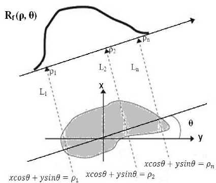
Fig.1: Radon Transform

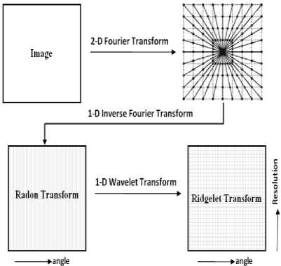
Fig.2: Ridgelet Transform

• V.    Methodology

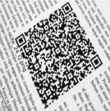
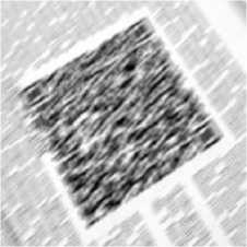
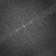
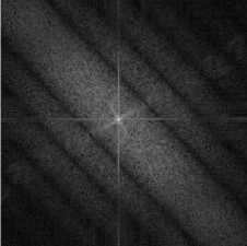
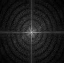
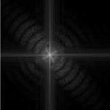
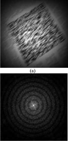
Blurring reduces significant features of image such as boundaries, shape, regions, objects etc., which creates problem for image analysis. The motion blur, defocus blur are appeared differently in frequency domain, and the blur categorization can be easily done using these patterns. If we transform the blurred image in frequency domain, it can be seen from frequency response of motion blurred image that the dominant parallel lines appear which are orthogonal to the motion orientation with near zero values [19, 20]. In defocused blur one can see appearance of some circular zero crossing patterns [21, 22] and in case of coexistence of both blurs combined effect of both blurs becomes visible. Fig.3 shows the effect of different blurs on the Fourier spectrum of original image. We can consider these patterns in frequency domain as image itself for blur classification. The steps of the algorithm to classify blur are detailed in fig.5. These are seven major steps: image acquisition, preprocessing of images, calculation of logarithmic frequency spectrum, feature extraction of blur pattern, data normalization, designing of neural network classifier system and result analysis.

(b)

(d)

(e)

(f)

Fig.3: (a) Original image containing QR code [24] (b) Motion blurred image (c) Fourier spectrum of original image (d) Fourier spectrum of blurred image with motion length 10 pixels and motion orientation 450 (e) Fourier spectrum of blurred image with defocus blur of radius 5 (f) Fourier spectrum of image with coexistence of both blurs

• A.    Preprocessing

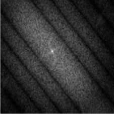
Blur classification requires a number of preprocessing steps. First, the color image obtained by the digital camera is changed into an 8-bit grayscale image. This can be made by averaging the color channels or by weighting the RGB-parts according to the luminance perception of the human eye. The period transitions from one boundary of image to the next frequently lead to high frequencies, which are converted into visible vertical and horizontal lines in the power spectrum of image. Because these lines may distract from or even superpose the stripes caused by the blur, they have to be removed by applying a windowing function previous to frequency transformation. The Hanning window gives a fine tradeoff between forming a smooth transition towards the image borders and maintaining enough image information in power spectrum. A 2D Hann window of size N X M defined by the product of two 1D Hann windows as w [n,m] = ^(1 + cos[27r^]).(1 + cos[27T^])    (12)

After this step, the windowed image can be transferred into the frequency domain by performing a fast Fourier transform. The power spectrum is calculated to facilitate the identification of particular features of the Fourier spectrum. However, as the coefficients of the Fourier spectrum decrease rapidly from its centre to the borders, it can be hard to identify local differences. Taking the logarithm of the power spectrum helps to balance this fast drop off. In order to obtain a centered version of the spectrum, its quadrants have to be swapped diagonally. In view of the fact that the remarkable features are around the centre of the spectrum, a centered portion of size 127 X 127 is cropped to perform ridgelet transform, which reduces computation time.

(c)

Fig. 4: (a)-(d) Hann windowed images of images shown in fig. 3(b), 3(d), 3(e) and 3(f).

(b)

X

(d)

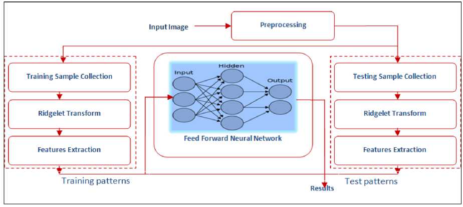
Fig 5: Blur classification framework

• B.    Feature Extraction

Finite Ridgelet Transform Toolbox (FRIT) [23] used for ridgelet transform. Implementation of FRT contains two main steps: application of a radon transform and an application a 1-dimensional wavelet transform. The radon transform was computed by first calculating the 2dimensional fast Fourier transform of the image, and then applying a 1-dimensional inverse Fourier transform on 128 radial directions of the radon projection. The radial directions were found using digital approximations. This approach captured exact samples from the image, however used approximate radial angles. Since the images were of size 127 x 127, 128 radial directions were extracted using digital approximations as described in [3]. A one-dimensional wavelet was applied to each of the 128 radial directions. The Haar wavelet is chosen for its superior discriminating power. In comparison to other wavelets, the Haar wavelet is theoretically straightforward and precisely reversible without edge effects. The Haar transform does not have overlapping windows, which reflects only changes between adjacent pairs of pixels. These features make them ideal for the use in the finite ridgelet transform. After achieving the ridgelet transform the mean and standard deviation of the coefficients related with each direction is calculated. The mean of a subband at orientation θ is calculated as

=    ^{( )}                       (13)

М+1                      v ’ where M x M is the size of image and E(9) is the energy of ridgelet transformed image respectively at orientation θ. Energy is calculated by the sum of absolute values of ridgelet coefficients as

Я (0 ) =Z^ _olR f (i,9)l              (14)

The standard deviation of a subband can be shown as

√∑    (|   ( , )|     )

, =

All these features are arranged in a manner such that the standard deviations remain in the first half of the feature vector and the means are arranged into the second half of the feature vector. So, we obtain a feature vector of size 256 consists of 128 mean energies and 128 standard deviations f = (f , f …, f ) for each of the power spectrum. We use this feature vector f to classify blur in different categories.

• VI. Simulation Results

  The image database used for the simulation is the Brno Institute of Technology QR code image database [24]. 350 images from the database were considered. Then, the three different classes of blur i.e. motion, defocus and combined were synthetically introduced with different parameters to make the databases of 1050 blurred images (i.e., 350 images with each class of blur). The classification is achieved using a feed forward neural network containing single hidden layer fifty neurons. Back propagation is pertained as network training principle where the dataset is designed by the extracted features of the blur patterns. The whole training and testing features set is normalized into the range of [0, 1], whereas the output class is assigned to zero for the lowest probability and one for the highest. During designing of neural network a cross-validation method is used to improve generalization ability. To carry out the crossvalidation procedure whole feature set is partitioned randomly into 3 sets training set, validation set and test set with a ratio 0.5, 0.2 and 0.3 respectively. The training set is used to learn the network. The validation set is used to validate the network i.e. to regulate network design parameters. The test set is used to test the generalization ability of the designed neural network.

In blur classification problem, we have used the four metrics for result evaluation given as

Number of true positive

PR   Total number of positive in dataset

Number of true negative

NR   Total number of negative in dataset

Number of false positive

FPR = Total number of negative in dataset

Number of false negative

FNR = Total number of positive in dataset

The aim of any classification technique is maximizing the number of correct classification given by True Positive Rate (TPR) and True Negative Rate (TNR), whereas minimizing the wrong classification given by False Positive Rate (FPR) and False Negative Rate. Terms True Positive (TP), True Negative (TN), False Positive (FP) and False Negative (FN) can be defined as below.

• (i) . True Positive (T P ) : In case of test pattern is positive and it is categorized as positive, it is considered as a true positive.

• (ii) . True Negative (TN): In case of test pattern is negative and it is categorized as negative, it is considered as a true negative.

• (iii) . False Positive (FP): In case of test pattern is negative and it is categorized as positive, it is considered as a false positive.

• (iv) . False Negative (FN): In case of test pattern is positive and it is categorized as negative, it is considered as a false negative.

The values of positive and Negative samples used as testing samples are 350 and 700, respectively for each blur categories. The data in Table I give the above discussed rates given by the classifier. Testing results give classifications accuracies as 98.2 %, 99.2 %, and 100% for motion, defocus and Combined blur categories respectively. Classification accuracy for each blur class is calculated as mean of true positive rate and true negative rate.

Table 1: Blur Classification results

Blur Type	Classification Results(in percentage)
	True Positive Rate	True Negative Rate	False Positive Rate	False Negative Rate
Motion Blur	96.6	100	0	3.4
Defocus Blur	100	98.3	1.7	0
Combined Blur	100	100	0	0
Motion Blur Classification Accuracy 98.2
Defocus Blur Classification Accuracy 99.2
Combined Blur Classification Accuracy 100

• VII. Conclusion

In this paper, we have proposed a new blur classification scheme for barcode images taken by cameras. The scheme makes use of the ability of ridgelet transform to discriminate blur patterns appear in frequency spectrum of blurred image. This work classifies blur in motion, defocus and combined blur categories, which can further help to choose the appropriate blur parameter identification approach for non-blind restoration of barcode images.

ACKNOWLEDGMENT