Brain Tissue Segmentation from the MR Images Affected by Noise and Intensity Inhomogeneity Using a Novel Linguistic Fuzzifier-Based FCM Algorithm

Magnetic resonance imaging (MRI) furnishes highly accurate information about the anatomical structure of the human brain in 3-D with high SNR. Various tissues present in the human brain can be discriminated very well with MRI. Hence it is the extremely preferred modality for the human brain diagnosis compared to others such as computed tomography, fluid attenuation inversion recovery, etc [1]. Brain tissue segmentation from MRIs is very important to deal with brain-related disorders. It finds applications in various medical diagnosis processes such as radiotherapy treatment planning, deep brain stimulation, and longitudinal monitoring for disease progression.

Brain tissue segmentation is a process of dividing the brain image to obtain vital brain tissues, such as white matter (WM), gray matter (GM), and cerebrospinal fluid (CSF). Various automated brain segmentation techniques are being suggested by researchers. The main process in these segmentation methods is grouping the pixels according to their intensity or spatial locations. The brain tissue structures are intrinsic and have poor and blurred boundaries which make the tissue segmentation hard.

Furthermore, the MR image primarily suffers from artifacts such as noise and bias fields also called IIH. These are added to the image during acquisition. The existence of these artifacts leads to significant misclassification of pixels for intensity-based segmentation methods which makes brain MRI segmentation a challenging task. Hence it is essential to remove such artifacts for the effective segmentation of brain MRIs.

There exist two classes of brain segmentation methods such as supervised and unsupervised. The supervised methods are fully automatic and use prior knowledge [2-7]. Unsupervised methods train themselves from the existing features by iteratively characterizing the properties of each tissue class [8-11]. Several optimization algorithms are also proposed for MR brain image segmentation [12-18]. Clustering is the best example of the unsupervised method in which pixels with homogeneous characteristics are classified into one cluster while pixels with different characteristics are classified into different clusters. Methods based on FCM clustering are the widely used techniques for MR brain image segmentation [10].

In the FCM-based clustering techniques, every pixel has its place in every cluster with varying degrees of membership values. The main limitation of the FCM is not considering the correlation between neighboring pixels while pixel classification. Thus, FCM segmentation is sensitive to artifacts such as noise and IIH. To reduce the effect of these artifacts and to increase the performance of the traditional FCM clustering procedure several approaches have been suggested in the literature for brain tissue segmentation. In [19], Ahmed et.al suggested a new FCM clustering method in which the standard FCM fitness function gets modified to segment the brain MRI by removing IIH. This technique consumes high time as it can deal with only single feature input at one time. A Markov random field (MRF) based FCM was proposed [20] in which noise sensitivity gets improved by filtering the image while clustering. But the noise removal is less as in this method spatial information is not incorporated and is applied to single-channel MRI or CT scan images. An adaptive FCM [21] was proposed for the 3-D brain MR images. This method considered spatial constraints in the form dissimilarity index to decrease the noise. However, this technique fails to segment the CSF region accurately. Chuang et..al [22] proposed a spatial FCM clustering technique for brain image segmentation. In this neighborhood information is integrated while deriving the membership function. But the computational complexity of the algorithm is more due to the randomly defined membership matrix. Guo et..al [23] proposed another adaptive FCM for brain image segmentation. In this noise gets eliminated by filtering and the filter parameters are calculated using the variations in the intensity levels of the considered neighborhood. This method used the standard FCM but failed to explain the effect of constant fuzzifier value while finding cluster centers. A conditional spatial FCM (CSFCM) technique was proposed [25] which is more sensitive to noise and IIH by incorporating an auxiliary variable into the membership function. The robustness and computational efficiency of the standard FCM can be improved by including spatial information while designing the fitness function [26]. A deviation-sparse-based FCM (DSFCM) [27] was proposed to evaluate the spatial correlation in the pre-defined neighborhood.

These described approaches do not give any solution for the noise caused because of the equidistant pixels and the uncertain values of the parameters related to fuzzy clustering. There is high dynamic range variation for MR brain images as the images are from different modalities and with different noise intensities and IIH. Hence fixed value for the fuzzifier (m) is not suitable for brain tissue segmentation. To make the fuzzifier more suitable for the brain image segmentation Interval Type-2 FCM (IT2FCM) and the general type-2 FCM (GT2FCM) [28, 29] were proposed. In IT2FCM fuzzifier has interval values [m_n m₂ ]. Both these techniques addressed the uncertainty involved in the fuzzifier but were not resolved. None of the previous methods used type-2 FCM for brain image segmentation. This point motivated us to improve the performance of the type-2 FCM so that it can handle brain image segmentation. This paper proposed a linguistic fuzzifier-based FCM (LFFCM) for tissue segmentation from brain MRIs. This is a modified type-2 FCM consisting of spatial information and adaptive weights. LFFCM reduces the uncertainty in clustering and constraints using an optimized member function that can be computed using the fuzzy value of the linguistic fuzzifier (M). Here finding membership values is less complex and a precise formula is introduced to partition the membership matrix.

In general, average filter is used before the clustering to have a spatial correlation between the pixels. Nonetheless, this methodology is appropriate for low-noise and single-feature input applications. Hence in this work, the Gaussian filter is employed to estimate the spatial information. If a pixel is at the same distance from multiple cluster centers then it has the same membership value for every cluster. These types of pixels are treated as noise pixels and are assigned zero or low membership values. The proposed technique uses an adaptive weight factor while calculating new cluster centers and assigns more weight to the pixel points that are very nearer to the estimated boundary. The performance of the proposed method is tested with BrainWeb and Internet brain segmentation repository (IBSR) databases [30, 31]. The outcomes are compared with some of the existing clustering methods such as fundamental FCM [21], Adaptive FCM (AFCM) [23], improved intuitionistic FCM (IIFCM) [24], fast and robust FCM (FFCM) [26], Interval type-2 FCM (IT2FCM) [28], and General type-2 FCM (GT2FCM) [29]. The rest of this article is organized as follows. Some of the state-of-the-art techniques are briefly explained in section II. The proposed method is presented in section III followed by the results and their discussion in section IV. Conclusions and future directions are presented in Section V.

• 2.    State-of-the-art Techniques

A. Fuzzy C-means (FCM)

FCM is the mostly used fundamental clustering procedure. In the FCM clustering approach, each pixel is allocated to multiple numbers of clusters with varying levels of membership value.

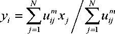
The image X = {x , x , . . . , x } with N number of pixels can be segmented into C number of clusters, using the fitness function [21]

Nc m2

fcm                   ij ij

=1 i =1

here u is the membership value of the pixel x in the i cluster with the center y . All the cluster centers are randomly selected initially and then updated. The term m represents the fuzzifier which is a real number greater than 1. d is the Euclidian distance between the pixel x and the cluster center y . The value of u can be found and updated utilizing the below equation (2) and has to satisfy the criterion in equation (3).

u _ij

{ uj

c

s

k = 1

Л m - 1 d ij

cN e [0,1]}/S uv =1Vjand0

The clusters are updated with each iteration as

This fundamental FCM is also known as Type-1 FCM. The algorithm is carried out with m = 2 and c = 3. The main drawback of FCM is that the pixel classification is done independently without taking spatial relationships among pixels into consideration. Hence segmentation using FCM clustering is sensitive to noise and IIH. Many FCM-based approaches are being proposed to handle the above limitation.

B. Adaptive FCM (AFCM)

This AFCM [23] is an improved version of the fundamental FCM. It includes the gray-level variance of the neighbͻring pixels into the fitness function. This method lessens the noise presented in the brain images and retains the original image resolution. The probability of occurrence of the local noise is used to design the fitness function and is given by

Nc

J afm = SX u m |[⁽¹ — Pj ) w j ⁺ P j x j ]^-У]\ j =1 i =1

where ̅ is the mean of the neighbors of the pixel . represents the weighted mean used to estimate the gray-level variance of the neighboring pixels. The probability of a pixel being a noisy pixel is calculated as

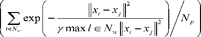
The terms N and N represent the neighbor window and the no. of pixels in that window respectively and γ is a scaling parameter. The equations used to update the membership function and cluster center are uij

II [(1 - p)

- 2/( m - 1) w j ⁺ P j x j J- ^-|

t [( ■ - p ) w j + P j x j J- у Г —° i = 1

cN

yj =t j [(1 - Pj) wj + PjXj} tum                       (8)

i =1                                                            i =1

• C.    Improved Intuitionistic FCM (IIFCM)

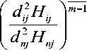
IIFCM [24] is another improved version of the type-1 FCM proposed to overcome the limitation of not having the exact boundary between different tissue regions. The fitness function is the same as that of type-1 FCM. This method uses an intuitionistic fuzzy factor to handle local spatial information. The intuitionistic fuzzy factor is defined as

H =—Z— i  Np ^ dkj+1

[ ( 1 - U j ) m + ( S j ) m J

For

Here S represents spatial membership value and the membership function is expressed as

u

ij

,1 <  i <  c ,1 <  j <  N

c t n=1

The centroid of the clusters is given by yj = min( p(yj ) q(yj ) r(yj ))                                (11)

where (  ),  (  ), and (  ) are the partial deriʋatives of the clusters’ Lagrange function. The main limitation of this technique is, that local spatial information is not incorporated into its membership value.

• D.    Fast FCM (FFCM)

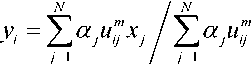
In this FFCM [26], the distance vector between the pixel and cluster center is replaced by fast membership filtering. The objective function can be minimized by using the Lagrange function for the pixel =    ( ) and its membership value . The term ( ) is to represent the morphological closing operation on the original image . The FFCM objective function can be expressed as

Nc

I

||xj - y i II- ^ t u j - ¹

V i = 1

m ffcm                    j ij j=1 i=1

here, α is a relative constant, and ∑ α ≤  . The term λ is a Lagrange multiplier which is to find the saddle point of the Lagrange function. The membership function and the cluster center are updated as

u

ij

xjyi

E c             - 2/( m - 1)

xj - yr r=1

This method uses both local and spatial information to enhance the segmentation results. Furthermore, the use of morphological operations improves denoising and information preservation.

• E.    Interval Type-2 FCM (IT2FCM)

In this IT2FCM [28], the fuzzifier value is calculated in a linguistic interval [   ,    ] rather than as a unique value.

This method is treated as Type-2 due to this advanced interval fuzzifier. As the fuzzifier is defined in an interval the membership values are also defined in an interval and are updated as

Uy = min

u₉,,. = max

2 ij

c

x j - y.

\ -2( m i -1)

c

x j - y

\ -2( m 2 -1)

xj - Ук xj - Ук

and the interval cluster positions are updated as

[ yi, У. ²] = Z ^u ( x i ) e J x

z

' ( x i >  J

Z x jj ^x j ) m

Z u ( X j ) )

By defuzzifying the interval centroid values, each cluster position can be calculated

y =

1        2

У¹ + У1

• F.    General type-2 FCM (GT2FCM)

The uncertainty associated while selecting the fuzzifier (m) in fundamental FCM can be resolved using GT2FCM [29]. In this a secondary membership matrix ̂ is constructed using a fuzzy linguistic fuzzifier (M) which can be expressed using α-cut representation as

M = U a B m ( O ) whereB M ( a ) = [ B^l_M ( a ), B M ( a ) ] a e[0,1]

The degree to which a pixel (x j ) belongs to the cluster (y_t) can be found using U as

[ Ui ⁽ x j ), U i ⁽ X j ^)] = Щ^] ^{a [} B . ⁽ x j / ^{a )} , B .⁽ x j I^{a )]}

where [ B ( (xj la), B $. (x j la)] are the boundary conditions for the interval linguistic fuzzifier [5 ^ (a), ^(a)].

The position of the centroid can be obtained as

C = U a [ C . ( a ), C .( a )] ui      a e [0,1]

Cluster center value depends on the centroid interval and can be obtained as:

A               /A

here Д is the discretization step number and z _t is the location vector of the discretized steps.

3. Proposed Method

A novel Linguistic Fuzzifier based FCM (LFFCM) is an extension of the GT2FCM technique. Determining the accurate position of the cluster is highly influenced by the uncertain value of the fuzzifier (m). The proposed method can overcome this limitation using linguistic relations. Using the α-plane representation the uncertainty present in the given image pixels is transformed into uncertain fuzzy partitions of the clusters extracted [32, 33]. Figure.1 depicts the flow diagram of the proposed linguistic process.

The algorithm is instigated by defining an interval for the fuzzifier range as [m_lf m ₂ ]. These are called values of the left and right fuzzifiers. Equation (19) is used to find the linguistic fuzzifier (M) in this defined linguistic interval. Then the left and right membership values of the type-1 FCM can be found using

U1ij = —

c

Z

к = 1

^U 2 ij

c

Z

к =1

A -2/ B M

x j ^- У к

X -2/ BM ( a )-1)

^XJ ^- У к

Then the spatial functions (   ,    ) that are used to represent the spatial information can be determined as

S,j = Z U„, S2j= Z  U2i.

^{k G} N m ^{( x} j )                ^{k G} N m ^{( x} j )

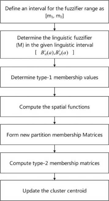
Fig. 1. Flow diagram of the proposed LFFCM

Here Nm(xj'r represents the neighborhood of the pixel x j and a window centered on pixel x j is used to represent the adaptive Gaussian filter. The Gaussian filter is adaptive in the sense that its order decreases concerning the convergence of the algorithm. The spatial functions (s1 j, s2 j) represent the probability of pixel Xj being in the cluster yt. New partition membership matrices can be obtained by integrating spatial information into the type-1 FCM membership matrix. The newly defined partition membership matrices (u^ j, uj^) are up

c z k = 1

pq u 1 kj s 1 kj

= U p

c z k = 1

pq u 2 kj s 2 kj

' ^u 1 ij

' u 2 ij

Here, the parameters p and q are used to accomplish the relative significance of both matrices [25]. These partition membership matrices and the interval fuzzifier values are used to define the type-2 membership matrices^ v1 (xj), v2(j')')- In the а-plane representation, the limits of the type-2 membership matrices are determined as v,.(x, / a) = min(u' , u ), 1i j                                        1ij        2ij

v _;( x_} / a ) = max( u ^ , u ₂₍.)

and the membership values are expressed as

Vi(Xj) = U a[Vii(Xj / a),v2i(Xj / a)]

a <0,1]

Now, the membership function (  ) of a pixel in the cluster can be obtained as vi = S vi(xj)

X j € X

The cluster centers are updated as

NN y=Swj(vi(xj))Mxj  Saj(v(x)M j=1

where w = ‖  -  ‖ signifies the adaptive weights estimated by finding the Euclidean distance between the pixel and the updated cluster center . In the concept of his adaptive weight, all the equidistant pixels are assigned to one cluster by taking into account the distance of the pixel closer to the expeϲted decision boundary.

This proposed type-2 LFFCM is found to be more effective in finding accurate cluster centers than the conventional FCM. It works well though the image is affected by noise and IIH. The convergence of the proposed method to erroneous local minima can be avoided by assessing the changes in the values of the fitness/objective function in subsequent iterations. The iteration should stop when the smallest improvement between the succeeding objective function values is lower than a prefixed error threshold. The concept of Defuzzification is employed to assign every pixel to a definite cluster according to its membership values. The fitness function of the proposed LFFCM is given by

Nc f=SS(v( x,)) “к- y,| f

j =1 i =1

The entire process of the brain MR image segmentation with the proposed method is presented as a diagram in Figure 2. The Brain MRIs used to test and analyze the proposed LFFCM algorithm are taken from the BrainWeb and IBSR database. MR brain image consists of both brain and non-brain tissues. Brain tissue can be extracted by removing the non-brain tissue region with the process of the skull- stripping. The presence of non-brain tissue leads to false segmentation. The skull-stripping technique used in this work is based on regional labeling and morphological operations [34]. The brain consists of three main tissues such as GM, WM, and CSF.

In the process of clustering using the proposed LFFCM, 3 clusters are chosen as there are three main brain tissues. Initially, the fuzzifier value is defined in a linguistic interval. Then linguistic fuzzifier (M) is calculated by utilizing the above interval linguistic fuzzifier values. Furthermore, the cluster centers are randomly initialized. After that, the type-2 membership values and the cluster centers are updated. Optimization of the proposed fitness function can be done using the process of iterative conditional mode optimization. In this procedure, all the equidistant pixels are allocated to the same cluster by assigning more weights to the pixels that are closer to the expected decision boundary. The proposed method works well for the removal of noise as it incorporates adaptive spatial information obtained from the neighborhoͻd of the pixels. Accurate convergence of the proposed method can be done by assessing the changes in the values of the objective function in subsequent iterations. The iteration should stop when the smallest improvement between the succeeding objective function values is lower than a prefixed error threshold. Conversely, the maximum number of iterations can also be considered as an alternative stopping criterion. Now, the brain MR image is divided into three clusters hence every pixel has membership values related to three clusters. The concept of defuzzification in which a pixel is assigned to a cluster where it has the highest membership value is applied to the membership matrix to acquire the brain tissue segments.

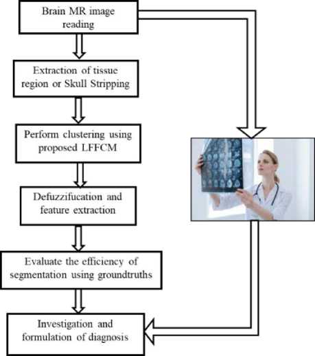
Fig. 2. Block diagram of the proposed LFFCM for brain tissue segmentation

• 4.    Results and Discussions

The performance of the proposed LFFCM is tested with both simulated and real MR Datasets. The simulated brain MR images are taken from BrainWeb [30] database and the real brain MR images are obtained from the IBSR [31] database. MATLAB is used to carry out the simulation. The performance is compared with various existing methods such as fundamental FCM [21], Adaptive FCM (AFCM) [23], improved intuitionistic FCM (IIFCM) [24], fast and robust FCM (FFCM) [26], Interval type-2 FCM (IT2FCM) [28], and General type-2 FCM (GT2FCM) [29]. Qualitative and quantitative analysis is done to validate the performance of the recommended approach. A detailed analysis of the results is presented in the subsequent subsections.

• A.    Simulated Brain MR Images

The Simulated brain database BrainWeb [30] consists of discrete anatomical models of GM, WM, and CSF. Each model comprises 181 slices, each of the size 181x217. The database offers different slice thicknesses, noise levels (0%, 3%, 5%, 7%, and 9%), and IIH levels (0%, 20%, and 40%). The model with noise and IIH of 0% is considered as groundtruths or the reference image. The noise present in the simulated image follows the Rayleigh distribution and the image is of the Rician distribution type. The % noise specifies the deviation of tissue intensity levels from their exact values owing to the white Gaussian noise. Likewise, 20% of IIH signifies an inhomogeneity in the range [0.90, 1.10].

The three different modalities of the MR images considered in this proposed work are T1-weighted, T2-weighted, and PD-weighted with different percentages of noise and IIH levels. Results are presented only for T1-weighted images. It can be observed that exact tissue regions are typically found in near middle slices of the total volume, hence these are considered for the experimentation. The performance of the proposed MR brain tissue segmentation method is compared with various existing methods such as fundamental FCM [21], Adaptive FCM (AFCM) [23], improved intuitionistic FCM (IIFCM) [24], fast and robust FCM (FFCM) [26], Interval type-2 FCM (IT2FCM) [28], and General type-2 FCM (GT2FCM) [29].

The segmentation results of the T1-w brain MR image are presented visually in Figure.3 to Figure.5. These results provide the qualitative evaluation. An image of 7% noise and 20% IIH is considered for the experimentation.

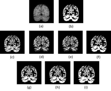
Fig. 3. Results of GM Segmentation. (a). Brain Image (b). Groundtruth (c)-(i). Results of FCM, AFCM, IIFCM, FFCM, IT2FCM, GT2FCM, and the proposed LFFCM respectively.

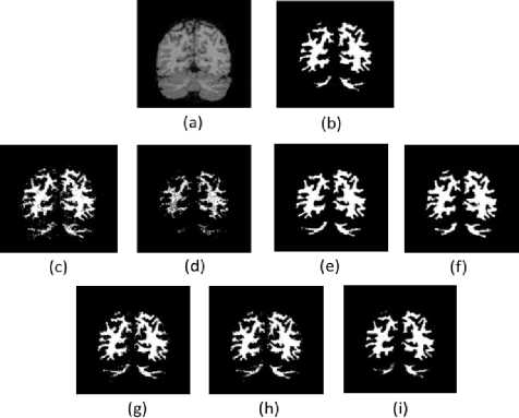
Fig. 4. Results of WM Segmentation. (a). Brain Image (b). Groundtruth (c)-(i). Results of FCM, AFCM, IIFCM, FFCM, IT2FCM, GT2FCM, and the proposed LFFCM respectively.

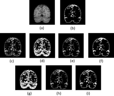
Fig. 5. Results of CSF Segmentation. (a). Brain Image (b). Groundtruth (c)-(i). Results of FCM, AFCM, IIFCM, FFCM, IT2FCM, GT2FCM, and the proposed LFFCM respectively.

From the figures, it can be observed that with high noise and IIH values fundamental FCM and its other alternatives are inept to segment the tissues accurately as noise and IIH still endures. In the segmented outputs of FFCM, various tissue regions are not noticeable due to less contrast in the images. There exists good contrast in the segmented results of IT2FCM and GT2FCM but the noise is not eliminated, hence tissue regions are not distinguishable. The results of the proposed LFFCM reveal that the three tissue regions are exactly segmented without having intersections of tissue regions. The results have less residual noise. These results appear to be very similar to groundtruth.

The results of all other methods are having intersecting tissue regions and showing traces of noise. The proposed method segmented the tissues accurately which are free from noise and IIH. The inclusion of adaptive weights in the spatial information of the fitness function of the LFFCM aims to determine the accurate cluster centers which result in noise-free output. Additionally, it can be observed that the quality of the image is improved proceeding from FCM to LFFCM.

The quantitative evaluation is carried out by finding the following performance parameters.

Dice Similarity Index (DSI): It is a widely used index. It indicates the similarity between segmented output (A) and reference image (B). It is computed as

^c

where and are the set of pixels from the segmented and the reference image respectively.

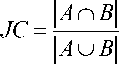
Jaccard Coefficient (JC): It is defined as the ratio of the intersection of segmented and reference images over the union of the same. It can be calculated as

Segmentation Accuracy (SA): It is expressed as the addition of the rightly classified pixels out of the total no. of pixels of the segmented image. It can be calculated as

_{SA =} у card (A ° B) ы \card ( Bk )|

where N indicates the total no. of pixels present in a cluster.

Tissue Sensitivity Analysis (TSA): It indicates the number of rightly classified pixels from the total no. of pixels in an image. It can be calculated as

TSA =    ^{2 N rcp}

^NRCP ^{+ N}PBG

where      is the number of rightly classified pixels,      is the total no. of pixels in the given image, and      is the number of pixels belonging to the groundtruth.

Partition Coefficient (PC): This denotes the degree of fuzzy partition between the clusters. It can be expressed as

cN ²

PC = ££ N i =1 j =1 ^N

Classification Entropy (CE): This indicates the degree of misclassification between the clusters. The formula to find CE is

cN

^-EE [ u j log u j ] i = 1 j = 1

N

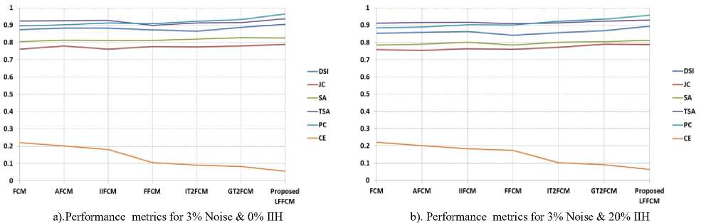
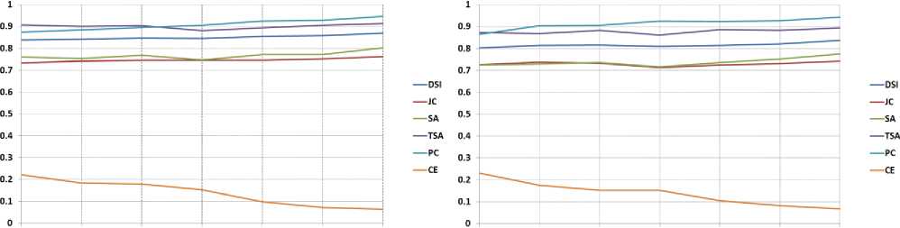
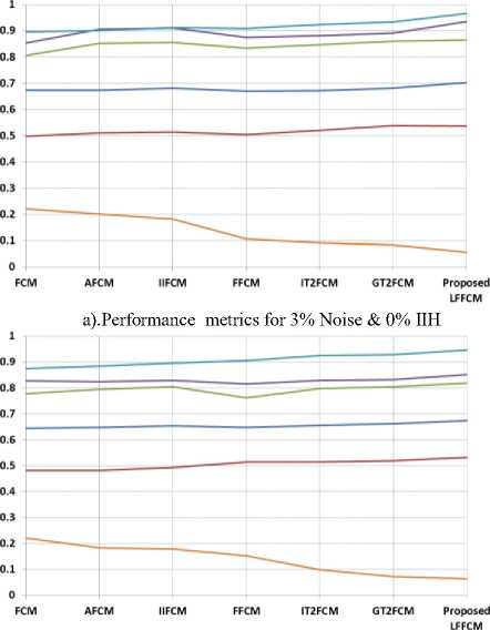
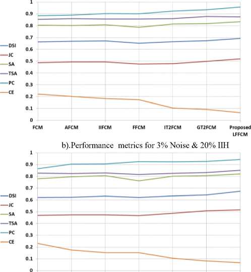
The optimal value of DSI, JC, SA, TSA, and PC is 1, the values nearer to 1 are better. The optimum value of CE is 0. Table 1 to Table 3 present the values of DSI, JC, SA, TSA, PC, and CE obtained by the proposed method and the other methods in segmenting GM, WM, and CSF from T1-w Brain MRIs. These indices are computed concerning to the groundtruth images. These indices values are the average values of 50 slices. The results are presented for various values of noise and IIH.

Table 1. Comparison of Performance Indices for GM Detection from T1-W Brain MR Images

Image	Method & Parameter	FCM	AFCM	IIFCM	FFCM	IT2FCM	GT2FCM	Proposed LFFCM
3% Noise & 0% IIH	DSI	0.8736	0.8824	0.8827	0.8730	0.8652	0.8865	0.9053
	JC	0.7611	0.7796	0.7609	0.7758	0.7734	0.7781	0.7884
	SA	0.8043	0.8127	0.8107	0.8112	0.8186	0.8274	0.8265
	TSA	0.9240	0.9252	0.9274	0.8992	0.9134	0.9144	0.9379
	PC	0.8954	0.9012	0.9124	0.9084	0.9228	0.9332	0.9654
	CE	0.2210	0.2014	0.1812	0.1062	0.0919	0.0838	0.0562
3% Noise & 20% IIH	DSI	0.8524	0.8572	0.8627	0.8408	0.8564	0.8672	0.8946
	JC	0.7583	0.7538	0.7624	0.7604	0.7706	0.7890	0.7868
	SA	0.7842	0.7884	0.8005	0.7845	0.8010	0.8042	0.8120
	TSA	0.9124	0.9145	0.9176	0.9079	0.9134	0.9232	0.9302
	PC	0.8846	0.8892	0.9016	0.8998	0.9238	0.9342	0.9584
	CE	0.2208	0.2018	0.1836	0.1738	0.1027	0.0912	0.0642
5% Noise & 0% IIH	DSI	0.8385	0.8412	0.8467	0.8442	0.8539	0.8586	0.8692
	JC	0.7342	0.7424	0.7448	0.7452	0.7451	0.7519	0.7622
	SA	0.7592	0.7524	0.7672	0.7468	0.7718	0.7712	0.8024
	TSA	0.9072	0.9011	0.9042	0.8808	0.8938	0.9047	0.9132
	PC	0.8742	0.8842	0.8958	0.9052	0.9258	0.9284	0.9464
	CE	0.2216	0.1842	0.1792	0.1522	0.0978	0.0718	0.0642
5% Noise & 20% IIH	DSI	0.8024	0.8131	0.8162	0.8096	0.8142	0.8208	0.8362
	JC	0.7252	0.7361	0.7324	0.7118	0.7241	0.7309	0.7422
	SA	0.7242	0.7284	0.7348	0.7152	0.7351	0.7519	0.7742
	TSA	0.8724	0.8672	0.8827	0.8608	0.8864	0.8832	0.8932
	PC	0.8642	0.9042	0.9058	0.9252	0.9228	0.9274	0.9428
	CE	0.2314	0.1754	0.1520	0.1528	0.1054	0.0826	0.0682
7% Noise & 0% IIH	DSI	0.7904	0.8024	0.8105	0.7854	0.8002	0.8038	0.8175
	JC	0.7201	0.7256	0.7249	0.7059	0.7134	0.7221	0.7384
	SA	0.7242	0.7314	0.7412	0.7248	0.7321	0.7409	0.7512
	TSA	0.8552	0.8621	0.8629	0.8458	0.8458	0.8664	0.8772
	PC	0.8652	0.8714	0.8884	0.8977	0.9254	0.9289	0.9375
	CE	0.2338	0.1818	0.1736	0.1228	0.0927	0.0872	0.0742
7% Noise & 20% IIH	DSI	0.7852	0.7789	0.7852	0.7832	0.7843	0.7939	0.8072
	JC	0.7022	0.7071	0.7124	0.7018	0.7082	0.7139	0.7222
	SA	0.7162	0.7124	0.7188	0.7152	0.7151	0.7249	0.7352
	TSA	0.8442	0.8435	0.8478	0.8352	0.8451	0.8562	0.8702
	PC	0.8642	0.8713	0.8738	0.8747	0.8954	0.9029	0.9307
	CE	0.2342	0.1834	0.1740	0.1238	0.1037	0.0864	0.0742

Table 2. Comparison of Performance Indices for WM Detection from T1-W Brain MR Images

Image	Method & Parameter	FCM	AFCM	IIFCM	FFCM	IT2FCM	GT2FCM	Proposed LFFCM
3% Noise & 0% IIH	DSI	0.8342	0.8514	0.8612	0.8497	0.8654	0.8689	0.8821
	JC	0.7424	0.7612	0.7544	0.7512	0.7647	0.7684	0.7824
	SA	0.8452	0.8624	0.8694	0.8725	0.8704	0.8842	0.9021
	TSA	0.8542	0.8712	0.8824	0.8678	0.8776	0.8734	0.8921
	PC	0.8954	0.9012	0.9124	0.9084	0.9228	0.9332	0.9654
	CE	0.2210	0.2014	0.1812	0.1062	0.0919	0.0838	0.0562
3% Noise & 20% IIH	DSI	0.8332	0.8324	0.8426	0.8235	0.8374	0.8502	0.8621
	JC	0.7422	0.7471	0.7514	0.7428	0.7531	0.7537	0.7608
	SA	0.8432	0.8442	0.8558	0.8562	0.8628	0.8754	0.8928
	TSA	0.8585	0.8507	0.8732	0.8648	0.8757	0.8912	0.9064
	PC	0.8846	0.8892	0.9016	0.8998	0.9238	0.9342	0.9584
	CE	0.2208	0.2018	0.1836	0.1738	0.1027	0.0912	0.0642

5% Noise & 0% IIH	DSI	0.8142	0.8123	0.8238	0.8217	0.8214	0.83029	0.9307
	JC	0.7240	0.7264	0.7312	0.7262	0.7335	0.7438	0.7562
	SA	0.8162	0.8126	0.8235	0.8042	0.8207	0.8327	0.8568
	TSA	0.8338	0.8317	0.8458	0.8216	0.8424	0.8532	0.8746
	PC	0.8742	0.8842	0.8958	0.9052	0.9258	0.9284	0.9464
	CE	0.2216	0.1842	0.1792	0.1522	0.0978	0.0718	0.0642
5% Noise & 20% IIH	DSI	0.7942	0.7998	0.8032	0.8002	0.8057	0.8138	0.8362
	JC	0.7242	0.7321	0.7314	0.7128	0.7251	0.7319	0.7434
	SA	0.7895	0.7996	0.8039	0.7858	0.8034	0.8169	0.8384
	TSA	0.8143	0.8167	0.8133	0.8042	0.8046	0.8232	0.8465
	PC	0.8642	0.9042	0.9058	0.9252	0.9228	0.9274	0.9428
	CE	0.2314	0.1754	0.1520	0.1528	0.1054	0.0826	0.0682
7% Noise & 0% IIH	DSI	0.7838	0.7864	0.7895	0.7745	0.7925	0.8032	0.8227
	JC	0.7121	0.7216	0.7279	0.7042	0.7034	0.7141	0.7336
	SA	0.7745	0.7786	0.7839	0.7678	0.7834	0.8069	0.8293
	TSA	0.8072	0.8041	0.8042	0.7908	0.8248	0.8347	0.8452
	PC	0.8652	0.8714	0.8884	0.8977	0.9254	0.9289	0.9375
	CE	0.2338	0.1818	0.1736	0.1228	0.0927	0.0872	0.0742
7% Noise & 20% IIH	DSI	0.7735	0.7746	0.7809	0.7848	0.7934	0.8057	0.8193
	JC	0.7072	0.7114	0.7183	0.7048	0.7071	0.7109	0.7212
	SA	0.7622	0.7641	0.7714	0.7618	0.7721	0.7819	0.7826
	TSA	0.7935	0.7975	0.8048	0.8014	0.8147	0.8162	0.8358
	PC	0.8642	0.8713	0.8738	0.8747	0.8954	0.9029	0.9307
	CE	0.2342	0.1834	0.1740	0.1238	0.1037	0.0864	0.0742

Table 3. Comparison of Performance Indices for CSF Detection from T1-W Brain MR Images

Image	Method & Parameter	FCM	AFCM	IIFCM	FFCM	IT2FCM	GT2FC M	Proposed LFFCM
3% Noise & 0% IIH	DSI	0.6732	0.6722	0.6812	0.6704	0.6712	0.6816	0.7032
	JC	0.4986	0.5104	0.5142	0.5052	0.5206	0.5382	0.5376
	SA	0.8052	0.8521	0.8539	0.8328	0.8472	0.8602	0.8652
	TSA	0.8538	0.9052	0.9104	0.8736	0.8809	0.8912	0.9342
	PC	0.8954	0.9012	0.9124	0.9084	0.9228	0.9332	0.9654
	CE	0.2210	0.2014	0.1812	0.1062	0.0919	0.0838	0.0562
3% Noise & 20% IIH	DSI	0.6624	0.6684	0.6715	0.6523	0.6643	0.6728	0.6922
	JC	0.4872	0.4922	0.4935	0.4753	0.4778	0.4972	0.5198
	SA	0.8046	0.8014	0.8079	0.7856	0.8137	0.8178	0.8327
	TSA	0.8537	0.8592	0.8556	0.8569	0.8597	0.8784	0.8742
	PC	0.8846	0.8892	0.9016	0.8998	0.9238	0.9342	0.9584
	CE	0.2208	0.2018	0.1836	0.1738	0.1027	0.0912	0.0642
5% Noise & 0% IIH	DSI	0.6437	0.6467	0.6538	0.6472	0.6554	0.6619	0.6732
	JC	0.4817	0.4812	0.4927	0.5146	0.5136	0.5189	0.5327
	SA	0.7785	0.7942	0.8047	0.7608	0.7972	0.8036	0.8187
	TSA	0.8262	0.8236	0.8289	0.8147	0.8286	0.8318	0.8508
	PC	0.8742	0.8842	0.8958	0.9052	0.9258	0.9284	0.9464
	CE	0.2216	0.1842	0.1792	0.1522	0.0978	0.0718	0.0642
5% Noise & 20% IIH	DSI	0.6214	0.6224	0.6315	0.6212	0.6343	0.6418	0.6722
	JC	0.4685	0.4727	0.4732	0.4668	0.4857	0.5082	0.5164
	SA	0.7787	0.7957	0.8062	0.7612	0.8012	0.8048	0.8197
	TSA	0.8264	0.8244	0.8292	0.8152	0.8254	0.8324	0.8512
	PC	0.8642	0.9042	0.9058	0.9252	0.9228	0.9274	0.9428
	CE	0.2314	0.1754	0.1520	0.1528	0.1054	0.0826	0.0682
7% Noise & 0% IIH	DSI	0.6144	0.6218	0.6245	0.6218	0.6319	0.6407	0.6626
	JC	0.4562	0.4593	0.4632	0.4667	0.4802	0.5012	0.5072
	SA	0.7742	0.7806	0.7892	0.7602	0.7757	0.7883	0.8062
	TSA	0.8125	0.8144	0.8152	0.8052	0.8214	0.8296	0.8412
	PC	0.8652	0.8714	0.8884	0.8977	0.9254	0.9289	0.9375
	CE	0.2338	0.1818	0.1736	0.1228	0.0927	0.0872	0.0742
7% Noise & 20% IIH	DSI	0.6124	0.6268	0.6255	0.6209	0.6312	0.6468	0.6583
	JC	0.4412	0.4531	0.4678	0.4428	0.4672	0.4702	0.4752
	SA	0.7632	0.7722	0.7635	0.7604	0.7724	0.7786	0.7842
	TSA	0.8343	0.8351	0.8269	0.8258	0.8282	0.8272	0.8562
	PC	0.8642	0.8713	0.8738	0.8747	0.8954	0.9029	0.9307
	CE	0.2342	0.1834	0.1740	0.1238	0.1037	0.0864	0.0742

FCM AKM IFCM FFM IT2FCM GT2FCM Proposed            FCM AFCM IIFCM FFCM IT2FCM GT2FCM Proposed

LFFCM                                                                                      LFFCM

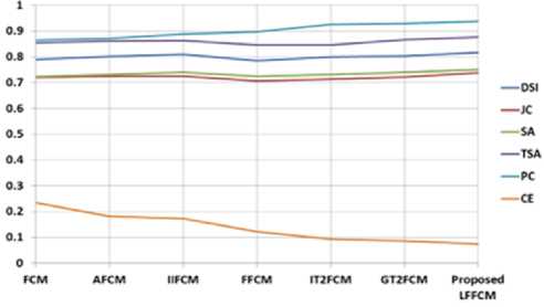
Fig. 6. Graphical Representation of performance indices for GM detection

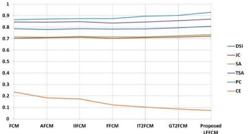
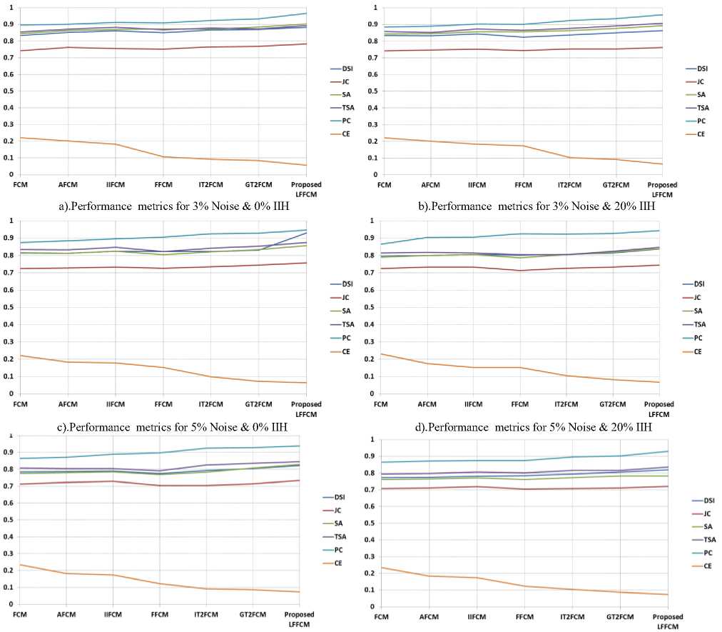
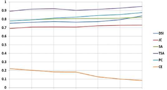
Fig. 7. Graphical Representation of performance indices for WM detection

---DSI

---JC

--ISA

--PC

--CE

---DSt

---JC

—SA

--TSA

—PC

—CE

FCM

AFCM

IIFCM

FFCM

IT2FCM

GT2FCM

Proposed LFFCM

---DSI

---JC

SA

—TSA

—PC

—CE

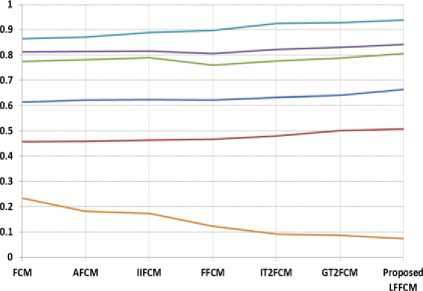
Fig. 8. Graphical Representation of performance indices for CSF detection

---DSI

---JC

--TSA

--PC

—CE

Table 4. Comparison of Performance Indices for T2-weighted Brain MR Images

Method & Parameter	FCM	AFCM	IIFCM	FFCM	IT2FCM	GT2FCM	Proposed LFFCM
DSI	0.7498	0.7632	0.7713	0.7635	0.7698	0.7914	0.8214
JC	0.6904	0.7084	0.7112	0.7096	0.7216	0.7275	0.7304
SA	0.7778	0.7824	0.8027	0.8076	0.8052	0.8126	0.8234
TSA	0.8916	0.9176	0.9224	0.9017	0.9124	0.9278	0.9536
PC	0.7805	0.7912	0.8126	0.8229	0.8415	0.8537	0.8736
CE	0.2214	0.2012	0.1816	0.1807	0.1246	0.1008	0.0826

Table 5. Comparison of Performance Indices for Pd-weighted Brain MR Images

Method & Parameter	FCM	AFCM	IIFCM	FFCM	IT2FCM	GT2FCM	Proposed LFFCM
DSI	0.7514	0.7634	0.7717	0.7642	0.7706	0.7917	0.8378
JC	0.6908	0.7078	0.7086	0.7074	0.7215	0.7283	0.7308
SA	0.7784	0.7924	0.8026	0.8078	0.8092	0.8112	0.8216
TSA	0.8926	0.9174	0.9216	0.9026	0.9132	0.9278	0.9486
PC	0.7796	0.7908	0.8124	0.8232	0.8436	0.8537	0.8756
CE	0.2218	0.2025	0.1832	0.1817	0.1262	0.1007	0.0832

Table 6. Comparison of Performance Indices with Real Brain MR Images

Method & Parameter	FCM	AFCM	IIFCM	FFCM	IT2FCM	GT2FCM	Proposed LFFCM
DSI	0.7833	0.7972	0.8063	0.8136	0.8230	0.8328	0.8492
JC	0.7342	0.7436	0.7455	0.7652	0.7675	0.7733	0.7842
SA	0.8113	0.8224	0.8432	0.8487	0.8532	0.8504	0.8812
TSA	0.8641	0.8854	0.8912	0.8842	0.8975	0.9012	0.9256
PC	0.7982	0.8214	0.8257	0.8169	0.8372	0.8582	0.9126
CE	0.2114	0.1872	0.1682	0.1134	0.1056	0.0862	0.0482

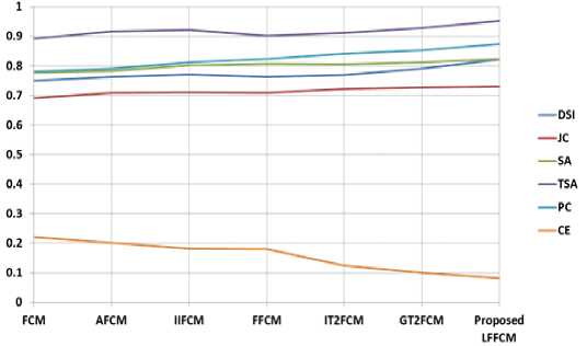
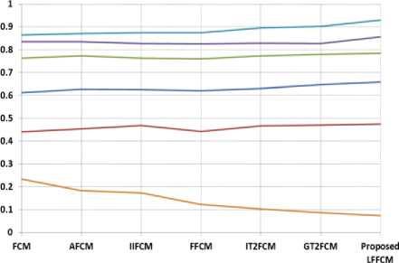
Fig. 9. Graphical Representation of performance parameters for T2-weighted Brain MRIs

FCM AFCM IIFCM FFCM IT2FCM GT2FCM Proposed IF FCM

Fig. 10. Graphical Representation of performance parameters for Pd-weighted Brain MRIs

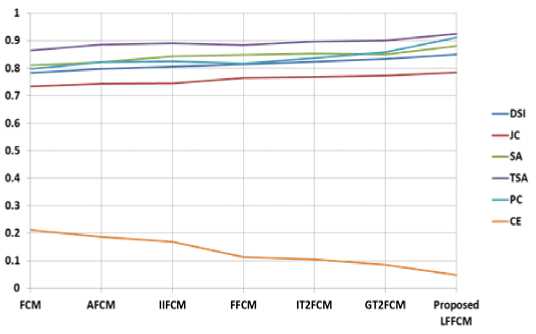
Fig. 11. Graphical Representation of performance parameters for Real Brain MRIs

• B.    Real Brain MR Images

• 5.    Conclusions and Research Implications

The proposed model is also validated using the clinically available normal images collected from the IBSR database. The IBSR database also provides groundtruth images used for the quantitative analysis. The proposed method also segmented real brain MR images more accurately with insignificant noise residuals. Table 6 shows the values of the performance indices computed by comparing the segmented image with the groundtruth. The values presented in the table are the average of all values obtained in segmenting the three tissue regions for the same values of noise and IIH added to simulated brain images. Figure 11 presents the graphical representation of the average performance parameters obtained during the detection of GM, WM, and CSF from Real Brain MR images for all the methods. The values presented are showing the excellent performance of the proposed method compared to some of the existing methods.

This work introduced a novel framework called Linguistic Fuzzifier based FCM (LFFCM) for the effective segmentation of GM, WM, and CSF from the brain MRIs which can also reduce the effect of noise and IIH simultaneously. The problem of equidistant pixels is solved by the proposed LFFCM. Here equidistant pixels are assigned to the same cluster by offering large weights to the pixels very nearer to the expected decision boundary. The effective Adaptive Gaussian filter is utilized to acquire spatial information. The order of the filter reduces when the algorithm is converged to final cluster centers. More accurate cluster centers are obtained compared to the conventional FCM even in the presence of noise and IIH due to the usage of this type-2 approach in computing membership values and cluster centers. In addition, the concept of α-plane representation employed in finding the linguistic fuzzifier (M) results in more accurate cluster centers. The values of segmentation evaluation parameters of qualitative and quantitative analysis using the proposed method indicate that this LFFCM outperforms the standard FCM, AFCM, IIFCM, FFCM, IT2FCM, and GT2FCM clustering techniques.

Though the method is outperforming some existing techniques it can be improved by including the best method for the estimation of IIH, removing partial volume effects, and considering 3D voxel instead of 2D pixel, etc.